From ADS-4 apps.dtic.mil.
Prerequisites
You need to have completed Aircraft Icing Handbook Energy Balance Examples.
Introduction
We will review "Engineering Summary of Airframe Icing Technical Data", ADS-4 apps.dtic.mil, as the anti-ice examples are more detailed than those in the "Aircraft Icing Handbook Volume 1", DOT/FAA/CT-88/8-1 apps.dtic.mil.
We will also look at "Ice, Frost, and Rain Protection", SAE AIR1168/4 sae.org, for practical guidance for analysis.
The ADS-4 and SAE AIR 1168/4 analysis methods use nomographs to implement graphical solutions. We will not be using the nomographs. While the notation is different, the analysis method from ADS-4 is very similar to the Standard Computational Model in the Aircraft Icing Handbook Merged Sections which we will use here.
The energy balance equation is:
Q"Source + Q"Sink = 0
Define Q"Sink by:

Q"Sink = Q"conv + Q"DropWarm + Q"Evap
Define Q"Source by:

Q"Source = Q"Freeze + Q"AeroHeat + Q"DropletKE + Q"IceCool
The only change required to the Standard Computational Model is the addition of heating:
Q"Source = Q"Freeze + Q"AeroHeat + Q"DropletKE + Q"IceCool + Q"Heat
For the usual case of anti-ice heating, the Q"Freeze and Q"IceCool terms are zero, but at low levels of heating they can be non-zero.
The heat balance is implemented in the file "thermal_anti_ice.py" (and associated files) available at github.com/icinganalysis/icinganalysis.github.io. Readers are encouraged to run the analysis to the duplicate results.
ADS-4 Method Description
3.5
3.5.1 THERMAL ANTI-ICING DESCRIPTION -
Thermal anti-icing systems use heat to maintain the temperature of the surface to be protected above freezing throughout an icing encounter. Thermal anti-icing systems are classified as evaporative and running wet.
Evaporative systems, as the name implies, supply sufficient heat to evaporate all water droplets impinging upon the heated surface.
The running wet systems, however, provide only enough heat to prevent freezing upon the heated surface. Beyond the heated surface of a running wet system, the water could freeze (generally called runback ice). For this reason, running wet systems must be used carefully so as not to permit runback ice buildup in critical locations. For example, the heated surface of a running wet system on a turboprop or turbojet inlet should extend into the inlet to the compressor face so that the water runoff will combine with the intake air and not strike cold surfaces where it could refreeze, break off, and possibly damage the engine.
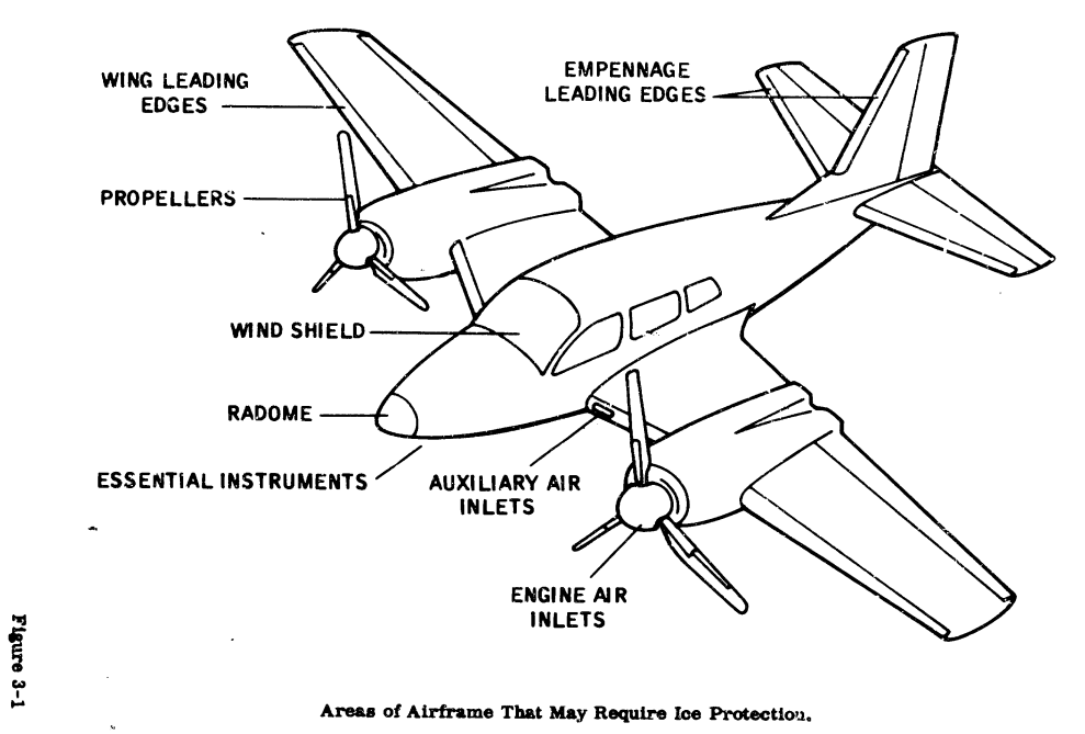
Basically, two sources of heat for thermal anti-icing are used in aircraft: electrical heaters and hot air. For anti-icing, the heat source must remain on throughout the icing encounter. Areas of an aircraft that may be afforded thermal ice protection are included in Figure 3-1. Of these areas, the windshield is always given anti-ice protection while the remainder of the areas may be given anti-icing or de-icing protection, depending on the power available for ice protection and the effects of ice accretion on the aircraft.
...
3.5.1.2 Hot Air System Description -
Several sources of hot air for anti-icing are available, depending on the aircraft type. engine bleed air may be available. In turbojet and turboprop aircraft, For piston engine aircraft, combustion heaters or exhaust gas heat exchangers may be used.
Areas usually protected by a hot air system are engine inlets, wing leading edges, and occasionally empennage leading edges. Basically, the hot air is manifolded to the various portions of the aircraft to be protected and finally distributed in any one of several methods, as shown in Figures 3-16 and 3-17. The hot air is introduced as close as possible to the stagnation point of the surface to be protected and permitted to flow chordwise toward an exit point through gas passages. The exhaust gas is generally dumped overboard at a non-critical location.
3.5.2
REQUIREMENTS -
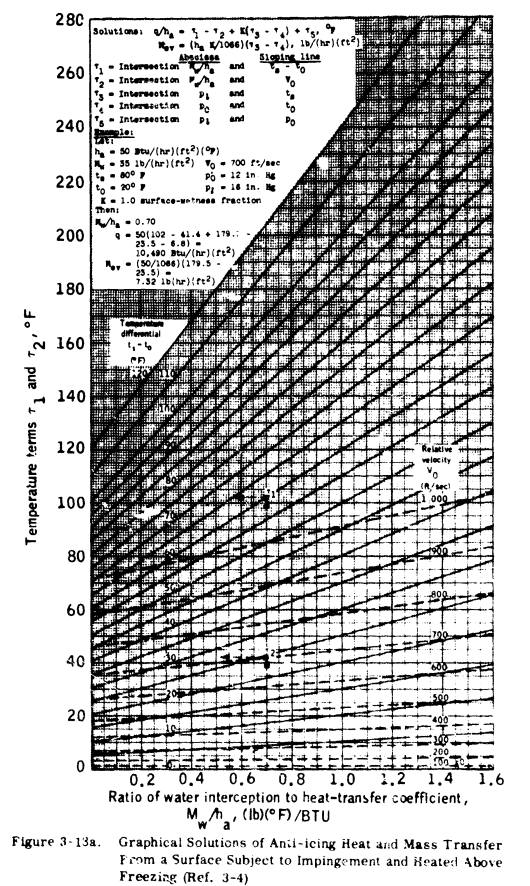
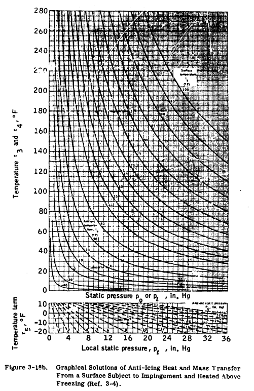
Equations expressing heat transfer and evaporation from wetted surfaces during icing encounters have been used to develop a graphical solution for the determination of heat required for anti-icing (Ref. 3-4). Figures 3-18a and 3-18b are presented for this purpose.
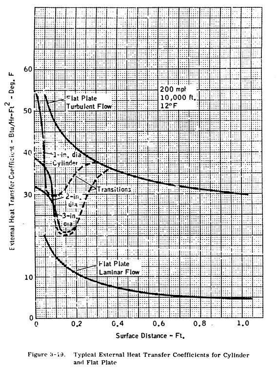
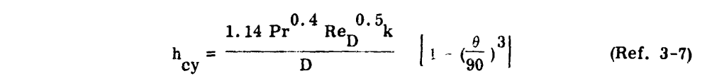
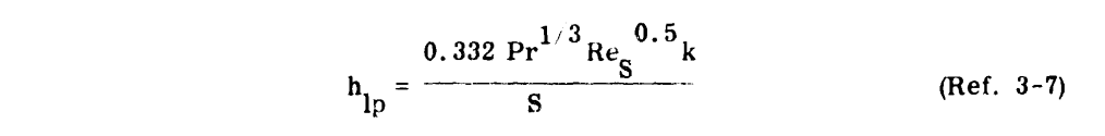
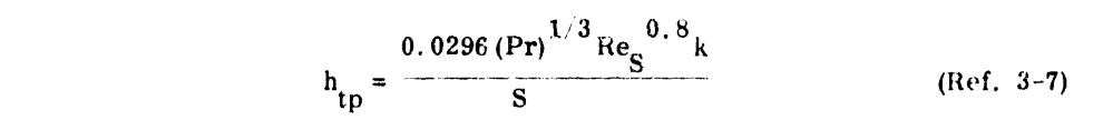
Preparatory to using these figures, the local heat transfer coefficient and rate of water catch (MW) must be determined. To determine the local heat transfer on an airfoil, the following three equations may be used:
a. Heat transfer coefficient for a cylinder (h_cy) of the same radius as the leading edge of the airfoil.
b. Heat transfer coefficient for laminar flow over a flat plate (h_lp) to the chordwise extent of the heated surface.
c.Heat transfer coefficient for turbulent flow over a flat plate to the chordwise extent of the heated surface.
A typical plot of these beat transfer coefficients is presented in Figure 3-19 for a specific altitude and airspeed.
The transitions from flat plate laminar to flat plat turbulent are only estimates, as the location of the transition region will vary with surface roughness, airfoil shape and angle of attack. Transition will usually start at a Reynolds Number of 0.5 to 2 x10^6 and the flow will be fully turbulent at a Reynolds Number of 2 to 4 x 10^6.
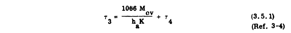
These equations may be used to determine the heat required per unit area along the chord. On tapered and swept-back airfoil, these calculations, performed at several span stations, can become unnecessarily tedious. In practice, the heat transfer coefficients for a span station are plotted as in Figure 3-19 and an average value assumed for that station. This average value (ha) is then used to enter Figures 3-18a and 3-18b to determine the anti-icing heat requirements. This assumption of an average value of heat transfer coefficient has a percentage of error in the same order of magnitude as the assumptions made in the meteorological variables.The water catch rate (Mw) is obtained by dividing the water catch (Wm) by the heated area per foot of span for each spanwise position (see Section 2 and the example in Section 4). For a completely evaporative system, the rate of evaporation of water (M_ev) must equal the rate of water catch (Mw). With this knowledge, the following equation may be solved for tau_3
If designing for a running wet system, the surface temperature (t_s) is assumed to be some value above freezing (such as 35 F), and tau_3 is found graphically.
The next steps are the graphical solution for tau_1 through tau_5 using Figures 3-18a and 3-18b and the solution of Equation 3.5.2 for the heat transfer rate at each spanwise position.
The heat transfer rate (q) may then be plotted versus spanwise position to obtain heating distribution requirements. Typical values for a wing are from 2,500 to 5,500 BTU/hr.-ft. span. [note: values corrected from "2,5000" and "5,5000".]


Practical simplifications
The method described in ADS-4 is not completely detailed, and relies on some engineering judgement.
Here, we will use some other recommendations to reach an analysis that is detailed enough to implement in a computer program.
Water catch rates
ADS4 briefly describes "airfoil matching" (using an airfoil that one has data for to approximate another airfoil), which is not used so much anymore.
The Aircraft Icing Handbook comments:
How was one to determine the impingement pattern for an airfoil not tested by the NACA? Before droplet trajectory and impingement codes were developed, one approach was to try to "match" the untested airfoil to one that had been tested and then "extrapolate" the impingement pattern (reference 2-22). [reference 2-22 is ADS-4]
By the early 1980's, many airfoils very different from those of the 1950's were in use or soon to be in use; for such airfoils, the "matching" procedure mentioned above was especially problematical. Furthermore, a need was recognized for impingement information on engine inlets and other three-dimensional configurations.
In conjunction with the need for new information, new technological possibilities also arose. ... There would no longer be any need for the difficult matching procedure.
SAE AIR1168/4 uses methods similar to the Aircraft Icing Handbook Water Catch Examples.
The water catch analysis methods we have seen previously, Aircraft Icing Handbook Water Catch Examples and Computer Impingement Analysis Tools Examples will be used here.
Surface Wetness Fraction
Unfortunately, ADS-4 does not detail the K term, "Surface wetness fraction", in equation 3.5.2 from NACA-TN-2799. Unfortunately, neither does NACA-TN-2799, beyond:
In the absence of exact data, the wetness fraction K in the basic equations is usually taken as 1 in the impingement area. Near the downstream limit of impingement, rivulets of run-back water commence and K decreases very rapidly. The K factors in regions of rivulet flow probably vary with many conditions, but limited data (reference 3) indicate that the value of K decreases in this region from a value near 0.3 down toward zero at the point of complete evaporation of run back.
"reference 3" of NACA-TN-2799 is NACA-TN-2480, which has more information, including this figure:
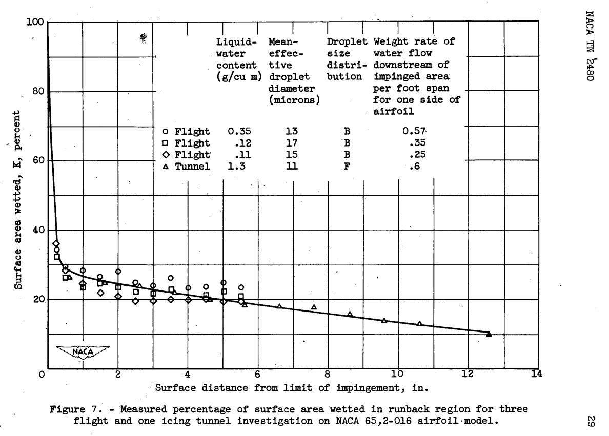
SAE AIR118/4 recommends simply using a value of 0.6 for K.
Here, we will calculate an average K value:
K = (1 * S_impingement + 0.3 * (S_heated-S_impingement)) / S_heated
Heat transfer coefficients
To implement the equations a, b, and c above,
engineering judgement is required
to approximately reproduce the values in Figure 3-19.
The recommended transition values do not well reproduce the figure.
The transitions from flat plate laminar to flat plat turbulent are only estimates, as the location of the transition region will vary with surface roughness, airfoil shape and angle of attack. Transition will usually start at a Reynolds Number of 0.5 to 2 x 10^6 and the flow will be fully turbulent at a Reynolds Number of 2 to 4 x 10^6.
The average value in Figure 3-19 is difficult to discern; I estimate it as 32 BTU/h-ft^2-F.
SAE AIR1168/4 uses the average flat plate turbulent flow heat transfer coefficient. The calculated average is 38 BTU/h-ft^2-F for Figure 3-19. SAE AIR1168/4 notes:
In all probability, an iced surface will be fully turbulent from the stagnation point.
A heat transfer text book 1 recommends:
... it would be unreasonable to expect the correlations to predict results to better than 25 percent accuracy
Here, we will use a +/-25% tolerance around the nominal heat transfer coefficient value. We will also consider the SAE AIR1168/4 turbulent flat plate method, which is often outside of the +/-25% tolerance.
Analysis zones
ADS-4 treats the heated surface as one analysis zone or control volume. This would include as one unit the upper and lower surfaces for a wing, for example, or the inner and outer barrels of an engine inlet. The protection requirements may be different for different surfaces, as the upper surface of a wing might be required to be fully evaporative, and different protection might be required for the lower surface.
SAE AIR1168/4 suggests using two analysis zones, split at the stagnation point:
the preceding equation accounts for the split of the water catch at the stagnation point; that is; half of the water is assumed for each top and bottom surface.
However, the water catch is not always split evenly at the stagnation point, so a more detailed analysis may be required, particularly at high angle of attack values.
Resources
-
"Engineering Summary of Airframe Icing Technical Data", ADS-4 apps.dtic.mil
-
"Ice, Frost, and Rain Protection", AIR1168/4 sae.org
-
"Aircraft Icing Handbook Volume 1", DOT/FAA/CT-88/8-1 apps.dtic.mil
Related
Back to Intermediate Topics
Citations
-
Incropera, F. P., De Witt, D. P.: "Fundamentals of Heat Transfer", John Wiley and Sons, 1984. ↩