Public domain image by Donald Cook.
Introduction
The "Aircraft Icing Handbook", DOT/FAA/CT-88/8-1, provides examples of two-dimensional water catch rates for the ice accretion process.
The Handbook uses something like "US Customary" or "Engineering" units in the calculations. This may limit the direct reuse of the equations.
These calculations can be reasonably accomplished through hand calculations, or a spreadsheet. However, they can be important "stepping stones" to build more complex capabilities.
Code written in the python programming language is available via github.com/icinganalysis, file "intermeadiate/basics_water_catch_calculations.py" (and associated files) for the solutions, under the LGPL license. Internally, the code uses (mostly) SI units (see A Brief Digression on Unit Systems for details). There are unit conversion functions in the python code. Values here are reported in the handbook units.
You are encouraged to run the provided code, or to start building your own library of such calculations (that will be far more instructional than just reading this text). The methods in the examples here may not seem very useful, given the current availability of more complex computing tools, but they provide quick and easy checks for those more complex calculations, that I have used for decades. They are also building blocks used to construct more complex calculations, such as those in the "Manual of Scaling Methods" NASA/CR-2004-212875, 2004 ntrs.nasa.gov.
Prerequisite reading
You should read, at minimum, these sections in the "Aircraft Icing Handbook", DOT/FAA/CT-88/8-1:
2.2.1.1 Droplet Trajectory Equation
2.2.1.2 Modified Droplet Inertia Parameter
2.2.1.3 Droplet Impingement Parameters
2.2.1.4 Droplet Size Distribution Effects
Note that the relevant sections in DOT/FAA/CT-88/8-1, 1991 apps.dtic.mil were affected by the perhaps little known update in 1993: apps.dtic.mil. The text here is from the updated version.
"Merged" text from the 1991 and 1993 update is available at Aircraft Icing Handbook Merged Sections
There are other sources with comparable information, but the notation from the Handbook will be used in the examples below.
Example 2-1
We will illustrate a solution of Example 2-1.
Example 2-1
An example of the calculation of Ko for an airfoil is now presented.
Airfoil:              c = 3.1 foot chord - NACA 0012
Flight Speed:         V = 200 kt (230.16 mph)
Altitude:             h = 10,000 ft (pressure altitude)
Ambient Temperature:  T = -4 F = 455.7 R
Droplet Size:         d = 20 microns
First find the air density and viscosity. From the pressure altitude, P = 1455.6 psf (10.109 psi). Solve for the air density using

For information on the archaic unit "slug", see A Brief Digression on Unit Systems.
A minor point is that DOT/FAA/CT-88/8-1 uses an approximation for the viscosity of air.
"μ" is the dynamic viscosity of air.
For viscosity, one can use the approximate relation:

This gives a result that is about 3.5% different from the viscosity equation used by Langmuir, which is a better approximation (using η for viscosity):

Now calculate Re and K.
In these units Re is given by
In these units K is given by:


If Langmuir and Blodgett's graphical method is used, the problem is completed by using figure 2-2. which shows that for Re = 126.8 the range parameter is approximately equal to .32. Then

Alternately, if Bragg's result is used, calculate Ko using Equation 2-10:

The difference in viscosity results in small differences in calculated values.
DOT/FAA/CT-88/8-1 Example 2-1 Calculation
mu handbook                : 3.252e-07
mu calculated              : 3.365e-07
mu fraction difference     :+0.035     ((calculated-handbook)/handbook)
K handbook                 : 1.554e-01
K calculated               : 1.502e-01
K fraction difference      :-0.033
Re_drop handbook           : 1.268e+02
Re_drop calculated         : 1.225e+02
Re_drop fraction difference:-0.034
Ratio handbook             : 3.200e-01
Ratio calculated           : 3.259e-01
Ratio fraction difference  :-0.018
Ko handbook                : 4.972e-02
Ko calculated              : 4.895e-02
Ko fraction difference     :-0.015
We will propagate the calculated Ko value into the next calculation.
Summarizing from the Handbook:
Summarizing this procedure for the usual case where the aircraft geometry, flight speed, pressure altitude, droplet size, and temperature are known:
1) From a standard atmospheric table obtain P from the pressure altitude, h. 2) Calculate the density (T in F):

3) Calculate the viscosity (T in F):

4) Solve for the droplet freestream Reynolds number.

5) Solve for the droplet inertia parameter

6) Use Re and K to calculate the modified inertia parameter using either equation 2-8 and figure 2-2 or else using equation 2-10.
Example 2-2
Example 2-2
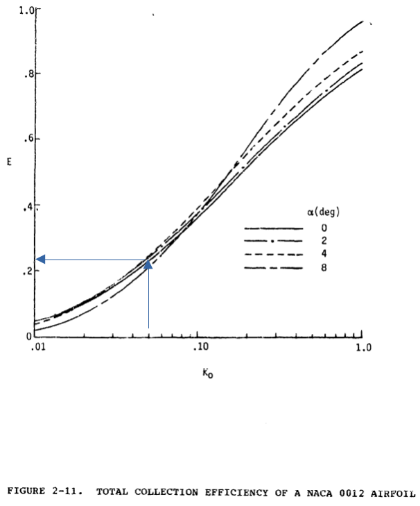
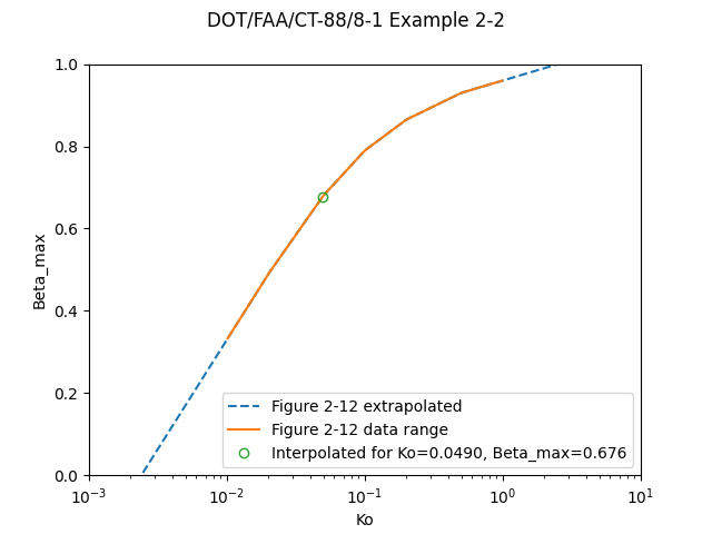
This example illustrates the estimation of the impingement parameters E, β, h, Su and SL using graphical data (reference 2-12). The graphical data is all presented with Ko as the independent variable. Much data is available in this form.The conditions of Example 2-1 for a NACA 0012 airfoil are assumed: thus Ko = 0.05. It also is assumed for simplicity that the angle of attack, α, is 0 degrees. From figure 2-11, E, the total impingement efficiency, is estimated to be 0.23 for these conditions. So about 23 percent of the water in the projected frontal area of the airfoil, with height h = .120c (found using figure 2-12), impinges on the airfoil. The maximum impingement efficiency for Ko = 0.05 and a = 0 degrees is estimated from figure 2-13 to be β_max = 0.68. At a = 0 degrees, the upper and lower limits of impingement are identical. From figure 2-14 at Ko = 0.05, SU = SL = .04. Therefore, water droplets will impinge on the airfoil leading edge only back approximately 4 percent of chord. (Note that this example assumes a "monodispersed" cloud, that is, a cloud in which all the droplets are of the same size. More realistic approaches are discussed in the following section.)
The solution for E and Beta (only) will be demonstrated here. Solving for the impingement limit is similar, and is left to the reader as a recommended exercise.
Example 2-2 may be solved graphically:
Public domain image by Donald Cook.
The figure can also be digitized and solved programmatically:
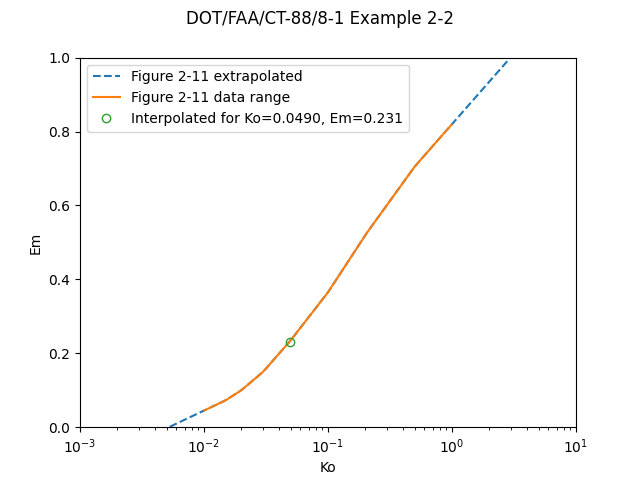
Public domain image by Donald Cook.
Public domain image by Donald Cook.
Example 2-3
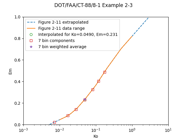
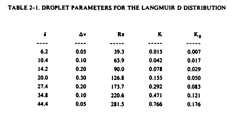
This example is a repetition of Example 2-2 except that this time the impingement parameters will be found using the entire droplet spectrum. It is assumed that the droplet median volume diameter (MVD) is 20 im (the droplet size used in Example 2-2) and the cloud droplet spectrum can be represented by a Langmuir D distribution. The droplet sizes representing the seven size bins in the distribution are calculated using table I-1 (discussed in Section 1.2.6). Table 2-1 shows the droplet sizes δ, the proportion δ_v of total droplet volume associated with each δ, and also the values of Re, K, and Ko for each δ.
Using these values of Ko and figure 2-11, a value E(δ) is associated with each δ, as shown in the third column of table 2-2. Note that equation 2-23 can also be written as

Thus E is calculated as an average value of the E(δ) weighted by volume using the Δv's. Table 2-2 shows that a value E = 0.24 is obtained, little different from the value E = 0.23 for the MVD. This is well within the accuracy of reading numbers from the figure.
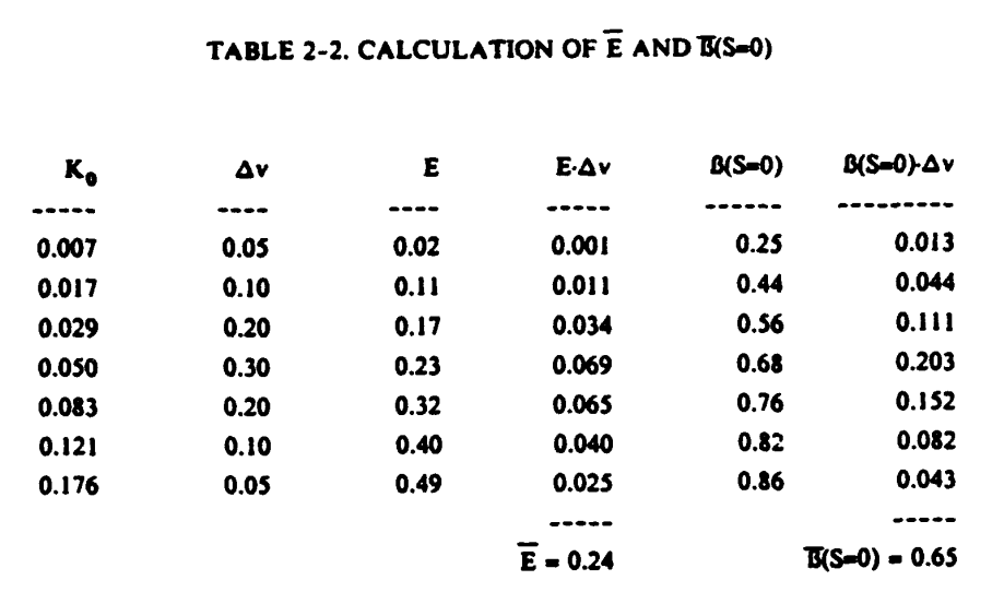
Considering this droplet size distribution and using equation 2-21, β_max can be calculated for a surface length location of S = 0 (stagnation point). For the special case of a symmetric airfoil at zero degrees angle of attack, where β_max occurs at S = 0 for all Ko, equation 2-21 can be used directly to determine β_max. In table 2-2 the calculation of β_max at S = 0 is summarized in the last two colum's, obtained from figure 2-11. Here again the value of β_max = 0.65 is close to the value for the MVD droplet size, where β_max = 0.68.
The maximum limits can be found from Ko,mas and figure 2-14. For the 44.4 micron droplet size, Ko,max =0.176 and from the figure SU = SL = 0.11, or 11 percent of the chord length. Estimates of the size of a pneumatic ice protection boot have been made by using an MVD of 20 microns and twice that diameter (40 microns) to determine the maximum extent of significant droplet catch. This comes to about 10% of the airfoil chord on the critical upper surface. Ten percent coverage of the upper surface is consistent with statistical measurements of upper surface icing made in the USSR (reference 2-13).
Comparison of Example 2-2 and 2-3 suggests that, except for the limits of impingement. impingement parameters calculated using the MVD may give a reasonably good approximation to those calculated over an entire droplet distribution.
This property of the MVD supplies the main justification for its wide use as the "representative" droplet size for a supercooled cloud in the study of aircraft icing. The error introduced in impingement calculations by its use rather than use of the full droplet spectrum is discussed in reference 2-14 and 2-15.
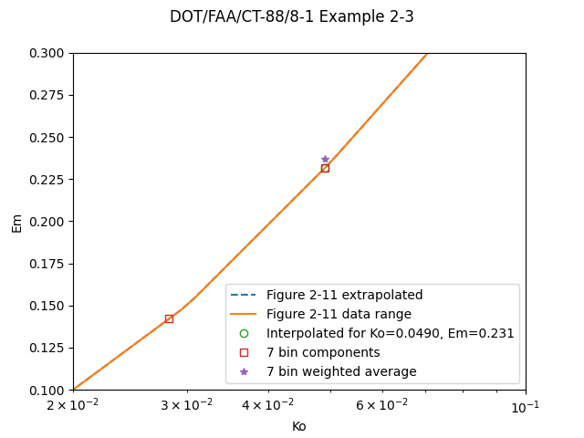
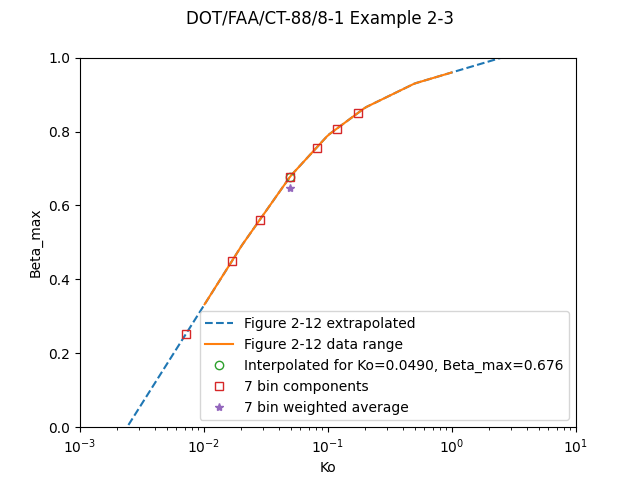
This example could be solved graphically and with by-hand calculations, but that is tedious. Here is a programmatic solution that yields similar values:
DOT/FAA/CT-88/8-1 Example 2-3 Table 2-2 Calculations
Ko       Δv    E      E*Δv  Beta  Beta*Δv
0.00710  0.05  0.021  0.001 0.251 0.013
0.01686  0.10  0.084  0.008 0.451 0.045
0.02813  0.20  0.142  0.028 0.561 0.112
0.04895  0.30  0.231  0.069 0.676 0.203
0.08096  0.20  0.325  0.065 0.756 0.151
0.11817  0.10  0.402  0.040 0.808 0.081
0.17296  0.05  0.488  0.024 0.849 0.042
̅E = 0.237
̅β = 0.647
The calculated E and β values differ slightly from the Table 2-2 values.
Here we can illustrate the weighted average solution.
Public domain image by Donald Cook.
If we zoom in we can see that the weighted average Em value is not necessarily on the curve developed for single drop sizes:
Public domain image by Donald Cook.
Public domain image by Donald Cook.
Example 2-4
The mass of ice accretion on the NACA 0012 section will be calculated. Using the same flight conditions as Example 2-1. and the droplet size distribution and value from Example 2-3:
Airfoil                         c = 3.1 foot chord NACA 0012
Flight Speed:                   V = 200 kt
Airfoil projected height:       h = 0.12 at alpha = 0
Liquid Water Content:           LWC = 0.4 g/m^3
Collection efficiency:          E = 0.24
Maximum impingement efficiency: Beta_max = 0.65
Icing time:                     tau = 5 minutes
Using equation 2-26 the mass of impinging water per unit span per unit time is given by:

Then for a five minute icing encounter (equation 2-27)

Calculating the accumulation parameter from equation 2-29 gives:
Note that the density of the ice is assumed to be 0.8 g/cm3. implying a rime accretion. The maximum ice thickness is approximated from equation 2-31 as


Thus the maximum ice growth is approximately 1.1 percent of the airfoil chord length, or about (.0106)(37.2) = 0.39 inches.
With the propagated values, the calculated final water catch rate from the python program differs by less than 1%.
DOT/FAA/CT-88/8-1 Example 2-4 Water Catch Span Rate Calculation
Reference value      : 0.0450 lbm/min-ft-span
calculated value     : 0.0446 lbm/min-ft-span
fraction difference  :-0.0091 (calc-reference)/reference
The calculated rime ice thickness differs by 0.8%.
DOT/FAA/CT-88/8-1 Example 2-4 Rime Ice Thickness Calculation
Reference value      : 0.390 inch
calculated value     : 0.393 inch
fraction difference  :+0.008 (calc-reference)/reference
Exercises
Reader are encouraged to perform the impingement limit calculations noted in Example 2-2 and Example 2-3. This will require programming data from the appropriate figures.
References (Handbook format)
2-2 Langmuir. I. and Blodgett, K., "A Mathematical Investigation of Water Droplet Trajectories," AAFTR 5418, February 1946. books.google.com
2-12 Bragg, M. B. and Gregorek, G. M., "An Analytical Evaluation of the Icing Properties of Several Low and Medium Speed Airfoils," AIAA Paper No. 83-109, January 1983. arc.aiaa.org
2-13 Trunov, 0., "Icing of Aircraft and the Means of Preventing It," English Translation, FTD-M7-65-490, p. 105, 1965.
2-14 Chang, H-P; Frost, W; Shaw, R. J.; and Kimble, K. R., "Influence of Multidrop Size Distribution on Icing Collection Efficiency," AIAA-83-0100, paper presented at the 21st Aerospace Scienzes Meeting, Jan. 1983. arc.aiaa.org
2-15 Papadakis, M.; Elangovan, R.; Freund, Jr., 0. A.; Breer, M.; Zumwalt, G. W..; and Whitmer, L., "An Experimental Method for Measuring Water Droplet Impingement Efficiency on Two- and Three-Dimensional Bodies," NASA CR 4257, DOT/FAA/CT-87/22, November 1989. ntrs.nasa.gov
Related
Back to Intermediate Topics