Introduction
The "Aircraft Icing Handbook" DOT/FAA/CT-88/8-1, 1991 apps.dtic.mil had a perhaps little known update in 1993: apps.dtic.mil.
Several errors and omissions were corrected in the update, so it is essential to consult the update.
As the update only include certain affected pages, it makes it difficult to read as there is much interruption paging back and forth between sources. Here, selected sections of the two sources are merged for easier reading.
The reproduction quality of the online sources is variable, and parts of the update are barely legible. Here, the text is used (not just scanned images of text). In some cases, I have included text of the equations.
Some readers may prefer the online web formatting over the pdf formatting. The figures are included inline, again to reduce paging back and forth. The cited references are also noted here. Links to online sources are provided, where available.
The merged texts are provided as a learning aid, they are not the authoritative source. You still have to consult both original source versions of the handbook to check for correctness and completeness of the merging done here. Not all sections have been merged.
The merged sections here do not use the block quote formatting to improve readability.
Water drop trajectories (transcribed text from DOT/FAA/CT-88/8-1 (updated 1993))
2.2.1.1 Droplet Trajectory Equation
(Section 2.2.1.1 and 2.2.1.2 are based primarily on reference 2-1, which draws heavily on the basic treatment of droplet trajectories presented in reference 2-2.)
The liquid water content of supercooled clouds rarely exceeds 1.0 grams of liquid water per cubic meter of air. This means that a cloud is rarely more than one-millionth liquid water by volume. Due to this low concentration of water droplets in the freestream, the flow way be considered uncoupled, meaning that the influence of the droplets on the flowfield can be neglected.
Supercooled water droplets in the atmosphere usually have diameters of less than 60 microns and experience Reynolds numbers small enough to permit their treatment as essentially spherical. (Although this is the universal computational practice, it has been argued that a droplet experiencing large accelerations in the vicinity of an ice accretion may assume a non-spherical shape which would alter its coefficient of drag and hence its trajectory (reference 2-3).)
Consider the trajectory of a single droplet approaching a body. The droplet trajectory equation is obtained by applying Newton's Second Law, F = ma, to the droplet. This equation can be expressed as

where x is the position vector of the droplet, t is time (the acceleration a is of course equal to the second derivative of x with respect to time), P is the pressure gradient term, M. is the apparent mass term, mg is the gravity force or "settling" term, B is the Bassett (unsteady) history force, and D is the drag force. The forces P and Ma are ordinarily neglected because the density of the particle (water droplet) is much greater that of the fluid (air) and the force mg can be neglected because of the very small mass of supercooled water droplets.
The force B accounts for the deviation of the flow pattern around the particle from that of steady state and represents the effect of the history of the motion on the instantaneous force (reference 2-4). It is essentially a correction to the drag term for an accelerating sphere. An accelerating sphere experiences a lower drag coefficient since it takes the flowfield some finite time to respond to the changing velocity and droplet Reynolds number.
The term is significant if the particle density is of the same order as that of the fluid (which is not the case here), or if the particle experiences "large" accelerations. Droplets experience their largest accelerations when in the leading edge region of an airfoil, and the accelerations are larger yet if "glaze horns" are present. Norment (reference 2-5), using the work of Keim (reference 2-6) and Crowe (reference 2-7), has argued that for the icing problem the accelerations experienced by the droplets are not large enough for the Bassett term to be significant. Lozowski and Oleskiw (reference 2-8) included the Bassett term in the droplet trajectory equation used in their droplet trajectory and impingement code (Chapter IV, Section 2). They state that their results suggest that "in most cases ... the term may be ignored without severely affecting the accuracy of the calculations" (reference 2-8, p. 11). The Bassett force will be neglected in the rest of this discussion.
The drag term, D, can be expressed as

u is the local flowfield velocity vector, S is the cross sectional area of the sphere (or the projected frontal area of the sphere), and CD is the drag coefficient. Note that the drag is evaluated using the velocity of the droplet with respect to the local airstream; this is sometimes called the "slip velocity." All the terms on the right hand side of equation 2-1 other than D are now dropped and equation 2-2 is used to substitute for D; this yields

where the equation has been divided by the mass m of the droplet, δ is the droplet diameter, and
ρw is droplet density and ρa is the air density.
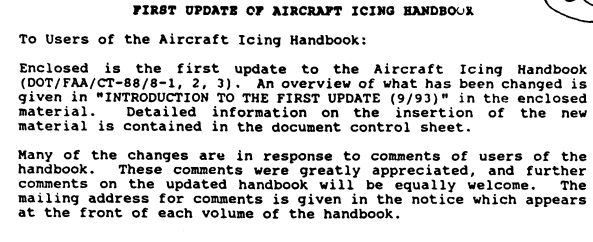
A standard drag curve (figure 2-1) for a sphere has been established by bringing together experimental results from many sources (reference 2-9). Only a limited range of this curve need be fit for supercooled water droplets, since the relevant droplet Reynolds numbers rarely exceed 500. A number of different fits are available, some of which are discussed in reference 2-1.
2.2.1.2 Modified Droplet Inertia Parameter {: #modified-drop-inertia-parameter }
Equation (2-3) will now be nondimensionalized in order to introduce the inertia parameter K and modified inertia parameter Ko (both further discussed in Chapter IV, Section 2). Letting x and y be the components of the vector x, define the nondimensional variables x = x/c, y = y/c, t* = t/(c/Vinf), where c is a characteristic length, t is time, and Vinf is the freestream airspeed. If the asterisks are suppressed after the equation is suitably rearranged, the nondimensional equation is

Now x_bar is the dimensionless droplet position vector, V_bar is the dimensionless local flowfield velocity vector, t is nondimensional time, Rel is the local relative droplet Reynolds number given by

(μs is the viscosity of air) and K is the droplet inertia parameter given by

It can be seen from equation (2-4) that the trajectory depends upon K and CDRel/24. But CDRel/24 can be shown (reference 2-2) to depend approximately upon Re, the free stream droplet Reynolds number which is given by

Therefore the droplet trajectory depends approximately upon Re and K only.
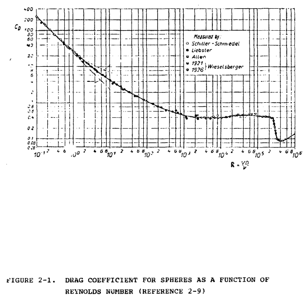
Langmuir and Blodgett (reference 2-2) combined Re and K into a single parameter Ko, referred to as the modified inertia parameter, as follows:

The quantity in brackets, referred to as the range parameter, is the ratio of the trajectory distance of a droplet in still air, with an initial Reynolds number of Re and gravity neglected, divided by the trajectory distance if the drag is assumed to obey Stokes Jaw. Using numerical methods, they obtained a graph giving the range parameter as a function of Re (figure 2-2).
Bragg (reference 2-10) has interpreted Ko by rewriting Equation 2-4 as

If some suitable average of the term in brackets on the left can be found over the entire trajectory, the droplet path becomes a function of just this single variable. Under typical icing conditions K. can be interpreted as such an average. Bragg also derived the following expression:

Equation 2-10 is shown in reference 2-1 to be within 1 percent of Langmuir's calculated values until Re approaches 1000 (much larger than the values for supercooled cloud droplets), where Langmuir's values diverge.
The approximate similarity parameter Ko has been introduced here because of its wide use in icing calculations. As shall be seen, it greatly simplifies the presentation of droplet impingement data. Ko will be further discussed in Chapter IV, Section 2, where ice scaling is addressed and where experimental and computational evidence will be presented in support of the use of Ko.
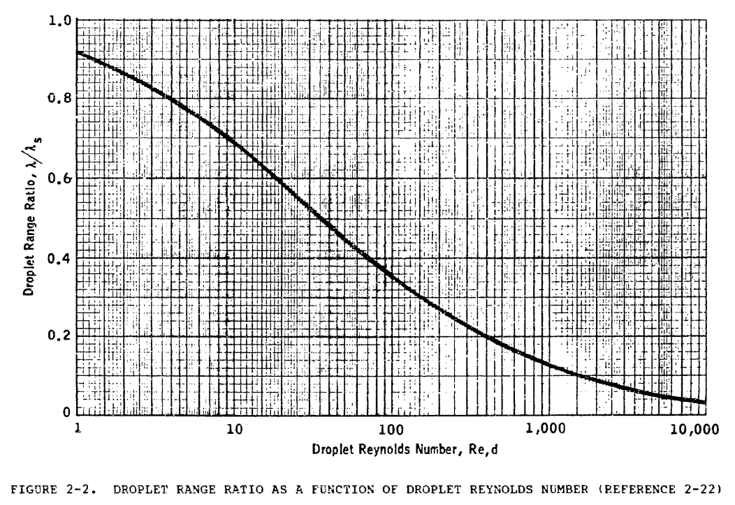
Ko can be interpreted as relating the importance of droplet inertia to the importance of droplet drag forces. For small values of Ko, drag predominates and the droplet tends to follow the flow streamlines until very close to the body. If Ko is small enough (approximately .005), the droplet acts approximately as a flow tracer. For large values of Ko, droplet inertia predominates and the droplet departs considerably from the flow streamlines as the body is approached. If Ko is large enough (approximately 1.0). the droplet trajectory is approximately a straight line that intersects the body. Figure 2-3 shows trajectories for two droplets approaching an airfoil, one with a diameter of 5 μm and Ko = .011 and the other with a diameter of 50 μm and Ko = .467. The trajectories were computed with the computer code LEWICE, which is discussed in Chapter IV, Section 2. Four chord lengths in front of the airfoil, the two trajectories are coincident (not shown in figure); however, they diverge dramatically in the vicinity of the airfoil due to the large difference in Ko between the two drops.
Bragg (reference 2-10) has derived another trajectory similarity parameter, K_bar, for which he has given a theoretical justification but which, nonetheless, has not as yet been widely adopted by other workers. Ko and K_bar are closely related and, differing by a constant factor if a simpe drag law is used in deriving Ko. Bragg shows that K_bar is given approximately by

It follows that since Ko approximates K_bar, Ko is approximately proportional to δ^5/3, to V^1/3, and to 1/c.
Figure 2-4 illustrates graphically values assumed by Ko under the range of MVDs and velocities that would ordinarily be experienced by a general aviation aircraft. The bottom panel is for a chord size representative of a full scale wing and the middle panel is for a chord size representative of a full scale horizontal stabilizer, both for a general aviation aircraft, while the top panel is for a chord size (6 inches) representative of an airfoil model. (Much research has been done with models of approximately this size, although larger models are generally preferred in tunnels which can accommodate them.)
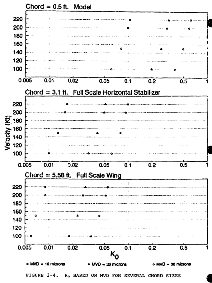
Comparison among the three panels shows that Ko is a strong function of chord size. In fact, the largest value of Ko for a full scale wing is approximately equal to the smallest value of Ko for the model. Examination of any one of the three panels shows that Ko varies strongly with MVD but much more weakly with aircraft velocity. All these observations are in accordance with equation 2-11. The reader may find it useful to refer back to this figure when studying the graphs presented later in which the impingement parameters E and β_max (defined in the next section) are presented as functions of Ko.
Figure 2-5 is constructed in the same manner, but using typical maximum droplet diameters rather than MVDs. It is interesting to note that the contrast among the three panels is now more pronounced due to the strong sensitivity of Ko to droplet diameter. Now the largest values of Ko even
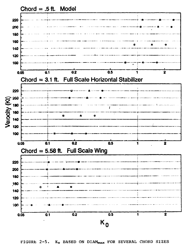
for a full scale horizontal stabilizer are substantially smaller than the smallest values of Ko for the model. This figure may be useful in interpreting the later graphs in which the impingement parameters Su and SL (defined in the next section) are presented as functions of Ko.
2.2.1.3 Droplet Impingement Parameters
Several impingement parameters can be defined to characterize the impingement properties of an airfoil or cylinder with respect to the cloud it encounters.
Figure 2-6 illustrates the definition of the impingement parameters Su, SL, ΔYo, h, and E for an airfoil in a supercooled cloud.
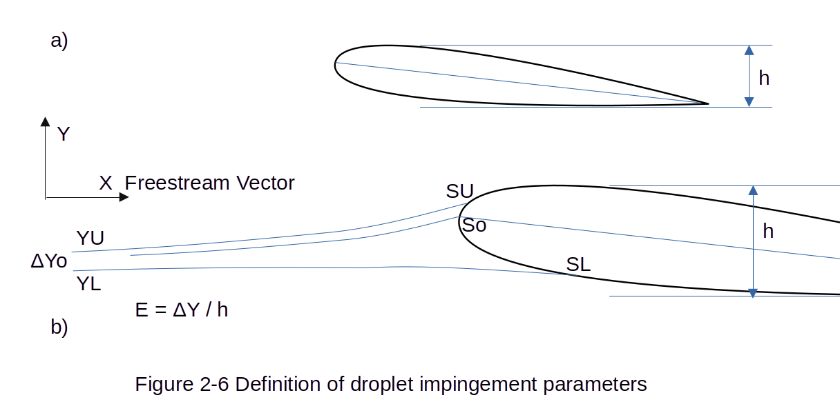
Figure 2-6 redrawn. Public domain image by Donald Cook.
Let S denote arc length measured along the airfoil surface. It is conventional to take S = 0 at the leading edge, and that is done here (although the reader should note that it is sometimes convenient to take S = 0 at the stagnation point instead). S is defined to be positive on the upper surface and negative on the lower surface. SU and SL are defined to be the upper and lower limits of droplet impingement on the airfoil and are determined by the upper and lower tangent droplet trajectories. Define a Y-axis that is perpendicular to the freestream velocity and far enough in front of the airfoil (at least several chords) so that the flow is essentially undisturbed by the presence of the airfoil; then the droplet trajectories can be taken initially to be parallel to one another and to the freestream flow lines. The droplet trajectory which strikes the airfoil at its leading edge intersects the Y-axis at a point which is taken to be Y = 0. The upper tangent trajectory intersects the Y-axis at a point YU and the lower tangent droplet trajectory intersects it at a point YL. Let ΔYo = Yu-YL; refer to this as the "freestream impingement width." Let h be the projected frontal height of the airfoil; note that this is a function of angle of attack. The total impingement (or collection) efficiency E is defined as the ratio of the freestream impingement width ΔYo to the projected frontal height h, i.e.,

E is the proportion of liquid mass crossing the Y-axis within the frontal projection of the airfoil and ultimately striking the airfoil.
In equation (2-16), E is a dimensionless quantity, but ΔYo and h are not. However, it is customary to nondimensionalize the latter two quantities by dividing them by the chord length c. A different notation is not ordinarily introduced for nondimensional ΔYo and h; in instances where the meaning may not be clear from the context, it is explicitly noted if the dimensional or nondimensional quantity is meant. Tables and graphs are available giving nondimensional ΔYo and h as functions of Ko and angle of attack α for some airfoils. Nondimensional ΔYo can be interpreted as follows: consider a segment of the Y-axis of length equal to one chord and centered at the projected position of the airfoil leading edge ΔYo is the proportion of liquid mass crossing the Y-axis within the segment which ultimately strikes the airfoil.
Figure 2-7 illustrates the definition of the local impingement (or collection) efficiency β at an arbitrary point P on the airfoil.
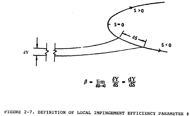
Let P lie between the points of impact on the airfoil surface of two droplet trajectories. The mass of water droplets between the two trajectories a distance SYo apart in the free stream (at the Y-axis) is distributed over a length δS on the airfoil surface. Letting δS approach 0 in such a way that P always falls between the impact points of the two trajectories, the local impingement efficiency 0 at P is defined in the limit by the derivative

The maximum value assumed by β anywhere on the airfoil surface is denoted by βmax. Note also that
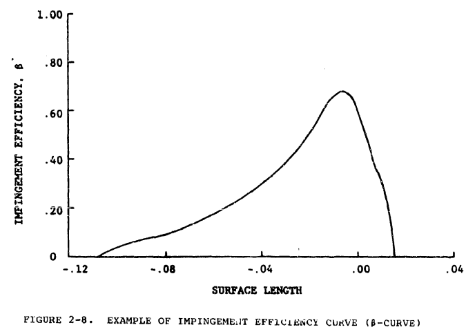
The impingement efficiency curve or β-curve is a plot of β on the vertical axis versus S on the horizontal axis. This is illustrated in figure 2-8.
The β-curve can be calculated numerically as follows: First, find the upper and lower tangent trajectories. These are ordinarily approximated numerically by finding upper and lower trajectories which pass within a small prescribed distance e of the airfoil without actually striking it. Second, calculate a set of trajectories between the upper and lower trajectories (figure 2-9).
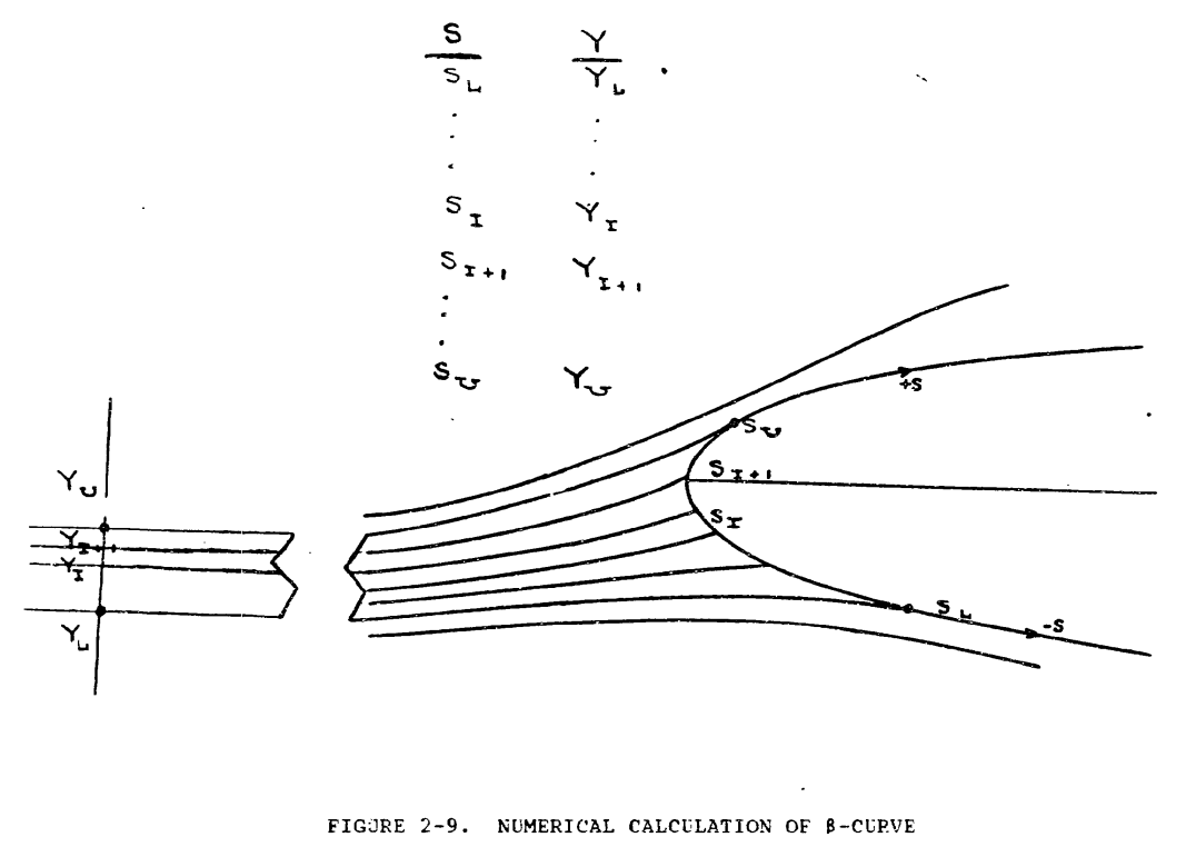
There is a Y value and associated S value for each trajectory. Third, fit a Y vs. S curve to the points (S, Y), as shown in figure 2-10.
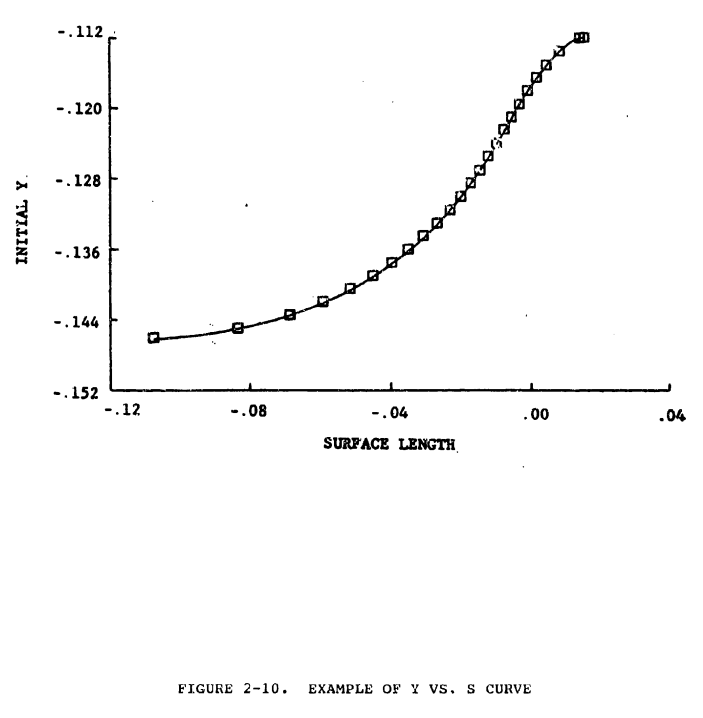
Fourth, approximate the derivatives to the Y vs. S curve at a set of points; these derivatives are the as. Fifth, fit a β-curve to the points (S, β). Some researchers omit step three and simply approximate βi for (Si, Yi) by the ratio (Yi+1 - Yi)/(Si+1 - Si), and then fit the β-curve to the points (Si, β).
As noted, equations 2-16 and 2-17 are for the two-dimensional planar case. The local impingement efficiency, β, can be calculated for the three-dimensional case by considering a three-dimensional tube of water droplets starting at infinity with some area, A, perpendicular to the freestream, and impinging on a body over some surface area, As. Then, the local impingement efficiency, β, is the limit, as As approaches zero, of A divided by As

Discussions of three-dimensional impingement calculations can be found in references 2-11 and 2-5.
2.2.1.4 Droplet Size Distribution Effects
The discussion thus far has proceeded as though clouds consisted of droplets of a single size ("monodispersed" clouds). All actual clouds, whether in the atmosphere or the wind tunnel, possess a spectrum of droplet sizes. This is taken into account in the definition of 0 and E by integrating over the droplet spectrum. In calculations with experimental data, this leads to taking averages weighted by volume, with the droplet spectrum represented by a histogram. Terms computed over the droplet spectrum are sometimes indicated by writing a bar above them.
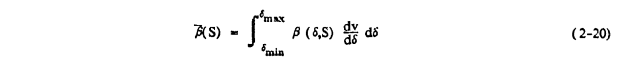
Here β_bar is called the droplet spectrum local impingement (or collection) efficiency at the surface position specified by S. The ph[r]ase "droplet spectrum" is ordinarily suppressed, since this is the meaning carried by the bar, some authors use the term "overall" rather than "droplet spectrum." The integral limits are the minimum and maximum droplet diameter in the cloud. In general, a droplet size distribution is described by v, the cumulative volume of water in the cloud as a function of droplet diameter, δ. In equation 2-20, the derivative of this curve, dv/dδ, appears. It is a function of the droplet size, δ, and, of course, the assumed cloud droplet distribution. Usually β and dv/dS are not known as continuous functions of δ and equation 2-20 is then represented as a summation
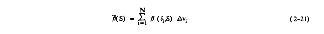
Equation 2-21 is summed over N discrete droplet sizes representing the midpoints of N droplet size bins. (For example, δi = 6.5 μm for a bin for droplets with diameters from 5 to 8 μm.) The droplet spectrum (or overall) impingement (or collection) efficiency E for an airfoil or body is defined in a similar way for a droplet size distribution:
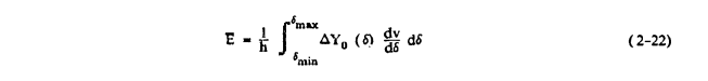
Here ΔYo(δ) is the initial Y difference for the tangent trajectories for a droplet of diameter δ. As in the case of β, one usually knows ΔYo (δ) for a discrete number of droplet sizes. Equation 2-22 can therefore be written as the sum

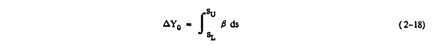
Note that a droplet spectrum (or overall) ΔYo may also be defined as

The limits of impingement depend not on the entire droplet spectrum but only on the largest droplets present in the spectrum. Let δmax denote the largest drop diameter present in the spectrum (or the midpoint of the bin containing the largest droplets), and let Ko,max denote the modified inertia parameter calculated using δmax. The maximum limits of impingement may be found from plots of Su and SL as a function of Ko_max, and angle of attack α.
[Several sections not included]
Energy Balance "Standard Computational Model" (transcribed text from DOT/FAA/CT-88/8-1 (updated 1993))
2.2.2.4 Physical Modeling of Ice Accretion Process
The physical modeling of aircraft icing consists of (1) the modeling of the trajectories and impingement of the supercooled water droplets and (2) the modeling of the behavior of the liquid water formerly in the droplets once it is on a surface of the aircraft. Part (1) has been presented above; the basic assumptions and equations go back to reference 2-2 and are widely accepted; discussion centers on the formulation of numerical procedures. Part (2), which will now be discussed, remains controversial. There exists what might be called a "standard computational model" which is incorporated in various forms in a number of computer codes, the most widely used of which is probably LEWICE (reference 2-39), developed under the direction of NASA Lewis Research Center.
However, a number of questions have been raised as to how accurately this model actually depicts the surface behavior of the liquid water. NASA-Lewis (reference 2-40) has initiated efforts to "formulate either changes to the existing model or an alternate model in order to see if ice shape predictions can be improved." (However, LEWICE can presently give useful ice shape predictions for a fairly wide range of conditions when used in conjunction with an appropriate roughness correlation; see the discussion in Chapter IV, Section 2.) This section begins with a presentation of the standard computational model; this is followed by a brief survey of the major criticisms of that model.
The standard model assumes that if air temperature is not low enough for impinging droplets to freeze upon impact, then the droplets are absorbed into a thin water film which flows away from the stagnation line (or point). As it flows, it is cooled mainly by convection to the airstream until it freezes, thus gradually changing the surface shape.
This model is formulated computationally by dividing the airfoil surface into segments, and associating a control volume with each segment. The water entering a control volume has two sources: (1) water droplets impinging on the surface segment; (2) water "running back" from an adjacent control volume closer to the stagnation point. (This "run back" water consists of all water which entered the adjacent control volume but did not freeze.) An energy balance analysis is applied to each control volume to determine the freezing fraction n, the fraction of the incoming water which freezes for that control volume. If n = 1, then all incoming water freezes. If n < 1, then a fraction 1-n does not freeze. This water will in turn run back into the adjacent control volume further away from the stagnation point.
The mass and energy balance analyses for a given control volume will now be presented in some detail. The energy balance analysis was given its classic formulation by Messinger (reference 2-41), whose work drew on earlier work by Tribus (reference 2-42). The presentation and notation used here is based on reference 2-43.
The mass balance for a control volume on the surface can be formulated as follows (figure 2-73).
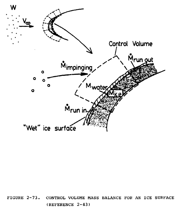
Let M"Imp denote the mass flux per unit time due to impinging water droplets, M"Run in and M"Run out denote mass flow per unit area per unit time into and out of the control volume due to liquid run back, and M"ice denote the mass of ice formed per unit area per unit time. Then the mass balance for the control volume is:
M"Ice = M"Imp + M"Runin - M"Runout - M"Evap

The term M"Imp is given by:
M"Imp = V∞ LWC β

V∞ is the freestream velocity. However, if the local velocity at the edge of the boundary layer is
available, that velocity should be used rather than the freestream velocity. This procedure is followed,
for example, in the ice accretion code LEWICE. β is the local collection efficiency for the control
volume.
It is convenient to define a term M"Incoming by:
M"Incoming = M"Imp + M"Runin

Then the freezing fraction n for the control volume is defined by:
n = M"Ice / M"Incoming
where M"ice is the incoming mass which freezes.
The energy balance for a control volume on the surface can be formulated as follows (figure 2-74).
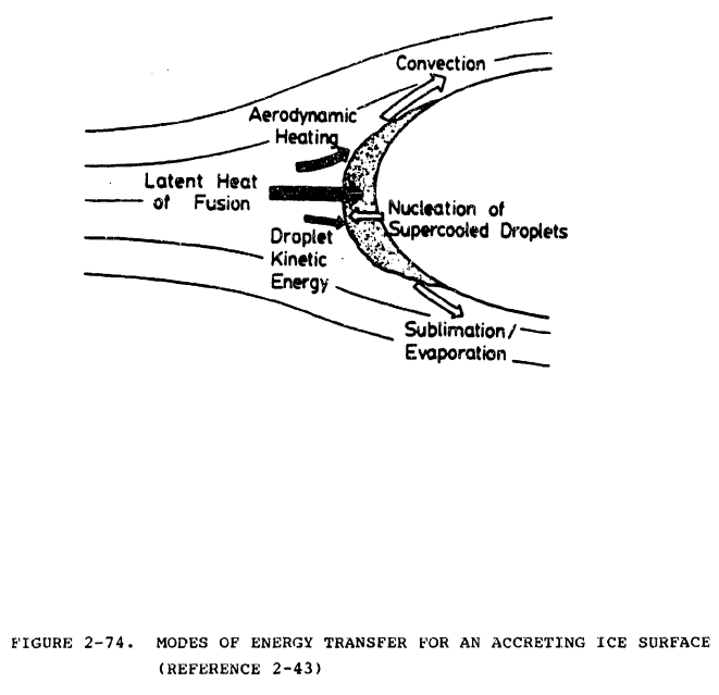
First, the main heat source terms (those that release heat into the control volume) are given.
Let Q"Freeze denote the freezing of the incoming water. Then
Q"Freeze = n M"Incoming Lf

where Lf is the heat of fusion.
Let Q"AeroHeat denote the aerodynamic heating. Then
Q"AeroHeat = hc rc V∞^2 / (2 CpAir)

where hc is the local heat transfer coefficient, rc is a recovery factor, and CpAir
is the specific heat of air.
Let Q"DropletK.E. denote the kinetic energy of the incoming droplets. Then:
Q"DropletKE = M"Imp V∞^2 / 2

Let Q"IceCool denote the cooling of the ice to the surface temperature TSurf. Then
Q"IceCool = n M"ice (Tf - Tsurf)

where Tf is the ice/water equilibrium temperature (32 F). Note that if n < 1, TSurf = Tf and so this term equals 0.
Define Q"Source by:
Q"Source = Q"Freeze + Q"AeroHeat + Q"DropletKE + Q"IceCool

Next, the main heat sink terms (those that remove heat from the control volume) are given.
Let Q"conv denote the convective cooling term. Then
Q"Conv = hc (Tsurf - T∞)

where T∞ is the freestream temperature. If the local temperature at the edge of the boundary layer
is available, that temperature should be used in this term rather than the freestream temperature. This
is also done in LEWICE.
Note: The term Q"Conv is often defined by
Q"Conv = hc (Tsurf - Tr)

where the "recovery temperature" Tr is given by
Tr = T∞ + hc rc V∞^2 / (2 CpAir)

In this formulation the term Q"AeroHeat is omitted from equation (2-41). In subsequent calculations
in this section, Q"AeroHeat is retained and equation (2-42) is used to calculate Q"Conv.
Let Q"DropWarm denote the droplet warming term. Then
Q"DropWarm = M"Imp Cw (TSurf - T∞)

where Cw is the specific heat of water.
Let Q"Evap denote the heat loss due to evaporation. There are a variety of formulations of this term. The approach used here is based on reference 2-44 and 2-U1 and employs the form of the Reynolds analogy.
M"Evap is given by
M"Evap = g ΔB

where g is the mass transfer coefficient and ΔB is the evaporative driving potential dependent on the
vapor concentration difference between the surface and the edge of the boundary layer.
These quantities are given by:
g = hc / CpAir (Pr/Sc)^0.667

ΔB = B1 / B2

B1 = PV,Surf / TSurf - (Po / P∞) (Pv,∞ / Ts)

B2 = 1/ 0.0622 (Po / To) - (PV,Surf / TSurf)
The Prandtl number Pr, Schmidt number Sc, and specific heat of air Cp air should be evaluated at the film temperature (To + Tsurf)/2. PV,surf is the vapor pressure at the surface and Pv,∞ is the free stream vapor pressure. The equations assume that Po and To the free stream pressure and temperature at the edge of the boundary layer are available; if they are not, the corresponding freestream values are used. 0.622 is the ratio of the molecular weight of water to that of dry air. The heat loss due to evaporation is now given by:
Q"evap = M"Evap Lv

Lv is the heat of vaporization.
If the freezing fraction is equal to 1 and the surface temperature Tsurf is to be computed, then Q"Evap should be replaced by the heat loss due to sublimation, denoted by Q"Subl. This is given by
Q"Subl = M"Subl Ls

where M"Subl denotes the mass flux due to sublimation per unit time and Ls denotes the heat of
sublimation. In some programs, M"Subl is computed using the same formulas as M"Evap.
Define Q"Sink by:
Q"Sink = Q"conv + Q"DropWarm + Q"Evap

The energy balance equation is:
Q"Source + Q"Sink = 0

The control volume freezing fraction is calculated as follows: Assume that the equilibrium temperature, Tsurf, is Tf. With this assumption, all quantities in the energy balance except n can be evaluated. Now solve for n. If the calculation yields a value of n between 0 and 1 inclusive, the calculation is complete. If n is calculated to be larger than 1, assume that n = 1 and that the excess over 1 was because Tsurf is actually smaller than Tf. So set n equal to 1 in the energy balance equation, which is now solved iteratively (since several quantities depend on Tsurf) for Tsurf. If n is calculated to be smaller than 0, similar reasoning leads to setting n equal to 0 and solving iteratively for Tsurf, which will now be larger than Tf.
A major source of uncertainty in calculating n using this equation arises from the uncertainty in the computation of the heat transfer coefficient h. If n is calculated in the stagnation region of a cylinder, it is common to use the heat transfer correlation for a smooth cylinder (given, for example, in reference 2-45).
If n is to be calculated in the stagnation region of an airfoil, the same correlation is sometimes used with radius equal to the radius of curvature of the airfoil. As the ice accretes, the shape changes and the surface roughness also changes, perhaps increasing dramatically. This can have a profound effect on the heat transfer coefficient.
Airfoil ice accretion codes must include an algorithm to calculate the heat transfer coefficient over the entire airfoil (See Chapter IV, Section 2). If it is a time-stepping code such as LEWICE, it must be able to calculate the heat transfer coefficient for an iced airfoil. An integral boundary layer method is typically used (See references 2-39 and 2-46). These methods generally include roughness terms, but a standard method for describing ice roughness has not yet been developed. NASA Lewis has conducted experiments to determine heat transfer coefficient distributions for ice shapes (references 2-47, 2-48). This data is essential to evaluate heat transfer coefficient algorithms. it appears that all existing algorithms introduce substantial uncertainty into the calculation.
References (Handbook format)
2-1 Bragg, M. B., "Rime Ice Accretion and Its Effect on Airfoil Performance," Ph.D. dissertation, The Ohio State University, 1981, and NASA CR 165599, March 1982. ntrs.nasa.gov
2-2 Langmuir. I. and Blodgett, K., "A Mathematical Investigation of Water Droplet Trajectories," AAFTR 5418, February 1946. books.google.com
2-3 Norment, unpublished.
2-4 Rudinger, G., "Flow of Solid Particles in Gases," ADARDograph No. 222, 1967, pp. 55-86. archive.org
2-5 Norment, H.G., "Calculation of Water Drop Trajectories to and About Arbitrary Three-Dimensional Bodies in Potential Airflow," NASA CR 3291, 1980. ntrs.nasa.gov
2-6 Keim, S. R., "Fluid Resistance to Cylinders in Accelerated Motion," J. Hydraulics Div. Proc. Amer. Soc. Civil Eng., Vol 6, 1956, paper 1113. ascelibrary.org
2-7 Crowe, C. T.; Nicholls, J. A.; and Morrison, R. B., "Drag Coefficients of Inert and Burning Particles Accelerating in Gas Streams," Ninth Symposium (int'l) on Combustion, Academic Press, 1963, pp. 395-405. sciencedirect.com
2-8 Lozowski, E. P. and Oleskiw, M. M., "Computer Modeling of Time--Dependent Rime Icing in the Atmosphere," CRREL 83-2, Jan. 1983. apps.dtic.mil
2-9 Schlichting, H., Boundary Layer Theory, McGraw Hill, New York, 4th Edition, 1960.
2-10 Bragg, M. B., "A Similarity Analysis of the Droplet Trajectory Equation," AIAA Journal, Vol. 20, No. 12, December 1982, pp. 1681-1686. arc.aiaa.org
2-11 Kim, J.J., "Particle Trajectory Computation on a 3-Dimensional Engine Inlet," NASA CR 175023 (DOT-FAA.-CT-86-1), January 1986 ntrs.nasa.gov
2-12 Bragg, M. B. and Gregorek, G. M., "An Analytical Evaluation of the Icing Properties of Several Low and Medium Speed Airfoils," AIAA Paper No. 83-109, January 1983. arc.aiaa.org
2-14 Chang, H-P; Frost, W; Shaw, R. J.; and Kimble, K. R., "Influence of Multidrop Size Distribution on Icing Collection Efficiency," AIAA-83-0100, paper presented at the 21st Aerospace Scienzes Meeting, Jan. 1983. arc.aiaa.org
2-15 Papadakis, M.; Elangovan, R.; Freund, Jr., 0. A.; Breer, M.; Zumwalt, G. W..; and Whitmer, L., "An Experimental Method for Measuring Water Droplet Impingement Efficiency on Two- and Three-Dimensional Bodies," NASA CR 4257, DOT/FAA/CT-87/22, November 1989. ntrs.nasa.gov
2-39 Ruff, G. A. and Berkowitz, B. M., "Users Manual for the NASA Lewis Ice Accretion Prediction Code (LEWICE)," NASA CR 185129, 1990. ntrs.nasa.gov
2-40 Shaw, R. J., "NASA's Aircraft Icing Analysis Program," NASA TM 88791, Sept. 1986. ntrs.nasa.gov
2-41 Messinger, B. L., "Equilibrium Temperature ef an Unheated Surface as a Function of Airspeed," Journal of Aeronautical Sciences, January 1953 (Vol. 20, No. 1). arc.aiaa.org [payment or institutional access required]
2-42 Tribus, M.V., et. al., "Analysis of Heat Transfer over a Small Cylinder in Icing Conditions on Mount Washington," American Society of Mechanical Engineers Transactions, Vol. 70, 1949, pp. 871-876. asme.org [payment or institutional access required]
2-43 "An experimental and theoretical study of the ice accretion process during artificial and natural icing conditions" DOT/FAA/CT-87/17 ntrs.nasa.gov
2-44 Analysis and Verification of the Icing Scaling Equations AEDC-TR-85-30 Vol. 1 (Revised)
2-45 Kreith, F., Principles of Heat Transfer, Intext Educational Publishers, New York, 1973, third edition archive.org [online borrowing with registration]
2-U1 Sogin, H. H., "A Design Manual for Thermal Anti-icing Systems". ADC Technical Report 54-313, Dec. 1954. ntrl.ntis.gov
2-46 Makkonen, L., "Heat Transfer and Icing of a Rough Cylinder," Cold Regions Science Vol. 10, 1985, pp. 105-116. cambridge.org
2-47 Van Fossen, G. J.; Simoneau, R. J.; Olsen, W. A.; and Shaw, R. J., "Heat Transfer Distributions around Nominal Ice Accretion Shapes Formed on a Cylinder in the NASA Lewis Icing Research Tunnel," NASA TM 83557, Jan. 1984. ntrs.nasa.gov
2-48 Poinsatte, P. E.; Van Fowsen, G. J.; and DeWitt, K. J., "Convective Heat Transfer Measurements from a NACA 0012 Airfoil in Flight and in the NASA Lewis Icing Research Tunnel," NASA TM 102448, Jan. 1990. ntrs.nasa.gov
Related
Back to Intermediate Topics