Public domain image by Donald Cook.
Prerequisites
To learn the energy terms and equations, readers should first review the "Standard Computational Model", which combines the applicable sections original DOT/FAA/CT-88/8-1 and the update into one text.
Introduction
The term "standard computational model" has not seen wide use. Most recent literature refers to the "Messinger Model" or "Modified Messinger Model". That may or may not mean the "standard computational model" presented here. As noted for calculating evaporation:
There are a variety of formulations of this term.
That could also apply to several of the terms in the model. "Modified Messinger Model" could mean about anything, you would need to look at the details.
The energy examples in the handbook are less detailed than the ones we previously saw for impingement.
The "Standard Computational Model" is implemented here in the python programming language and is available via github.com/icinganalysis, file "intermeadiate/table_2_5.py" (and associated files) for the solutions, under the LGPL license. Internally, the code uses (mostly) SI units (see A Brief Digression on Unit Systems for details). There are unit conversion functions in the python code. Values here are reported in the handbook units.
Aircraft Icing Handbook Table 2-5 Example
Dependence of freezing fraction on meteorological and flight variables
The dependence of the freezing fraction n on meteorological and flight variables in the standard computational model will now be illustrated by calculations at the stagnation line of a circular cylinder of diameter 20 cm. The calculations were done using a program that is a modification of the one discussed in reference 2-44. This program uses the heat transfer coefficient correlation for a clean cylinder from reference 2-45. If these calculations were done for a different geometry, or with a different program, or using a different heat transfer coefficient correlation, the numerical values would certainly change, but the general relationships illustrated would be much the same. Two "baseline conditions" are specified:
          Ambient           Droplet  Freestream
          Temperature LWC   Diameter Velocity
Condition  C          g/m^3 um       Vinf (m/s)
a.        -26         0.7   20       70
b.         -6         0.1   20       70
These were chosen because both have a freezing fraction of approximately .9 and both permit the variation of each of the four parameters individually, driving the value of n toward 0.
(It must be emphasized here that the following results indicate the magnitude of the freezing fraction along the stagnation line only. The unfrozen water may run back (or "slide" back in the form of large surface drops) from the stagnation line and eventually freeze somewhere on the cylinder. This is discussed further in the next section.)
Starting with condition (a), n was calculated for several increasing values of Tinf terminating with -2 C (figure 2-75a) and then the same procedure was followed starting with condition (b), again terminating with Tinf = -2 C (figure 2-75b). The figures illustrate that n decreases linearly with increasing T. Note that figure 2-75a, with a relatively large LWC of .7 and starting from a low temperature of -26 C, exhibits a much slower rate of decrease in n than does figure 2-75b, which has a LWC of .1 and starts from a much higher temperature of -6 C.
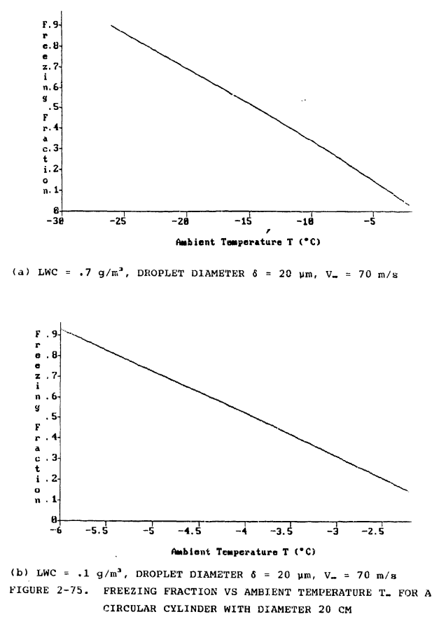
Table 2-5a shows the relative contributions to the energy balance of the main heat source and heat sink terms for condition (a) as T increases. For the source terms, the relative contribution of the droplet freezing term falls dramatically as the freezing fraction approaches 0 and this results in a larger relative contribution of the aerodynamic heating term. For the sink terms, the contributions are relatively constant. Table 2-5b for condition (b) shows that because LWC = .1 the relative contribution of the droplet freezing term is smaller at all temperatures and the relative contribution of the aerodynamic heating term is correspondingly larger. For the sink terms, the contributions are again relatively constant.
Table 2-5. Percentage contributions of main terms in energy balance
           for increasing Tinf for a circular cylinder with diameter 20 cm

           (a) LWC = 0.7 g/m^3, droplet diameter 20 um, Vinf = 70 m/s

           Percentage of
           Heat source terms             Heat sink terms
           Aerodynamic Droplet  Droplet  Convective Evaporative Droplet
 TC  N     heating     freezing KE       cooling    cooling     warming
-26  0.9    5          94        1       48         16          36
-20  0.7    6          93        1       47         18          35
-14  0.49   8          91        1       46         21          33
 -8  0.27  14          84        2       44         24          32
 -2  0.03  53          38        9       44         25          31

           (b) LWC = 0.1 g/m^3, droplet diameter 20 um, Vinf = 70 m/s

           Percentage of                                                ```
           Heat source terms             Heat sink terms
           Aerodynamic Droplet  Droplet  Convective Evaporative Droplet
 TC  N     heating     freezing KE       cooling    cooling     warming
 -6  0.93  24          75        1       60         16          36
 -4  0.53  36          63        1       47         18          35
 -2  0.10  73          25        2       46         21          33
Reproducing the examples
Figures 2-75 through 2-78 and Tables 2-5 through 2-8 show an example analysis for a 20 cm diameter cylinder in a range of icing conditions.
(Other results tables and figures not included here.)
The examples are useful for showing general trends and relative percentages of energy.
For comparison, I have implemented the "Standard Computational Model" in the python programming language.
Not all analysis details were described. For example, an altitude or air pressure was not noted. I assumed a sea-level altitude. A drop size distribution was not defined. I assumed a "Langmuir A" distribution (single or mono-dispersed drop size).
The method of determining the leading edge stagnation line water catch β value is not defined in the handbook text. For the calculations here, the cylinder line from Figure 2-43 is used.
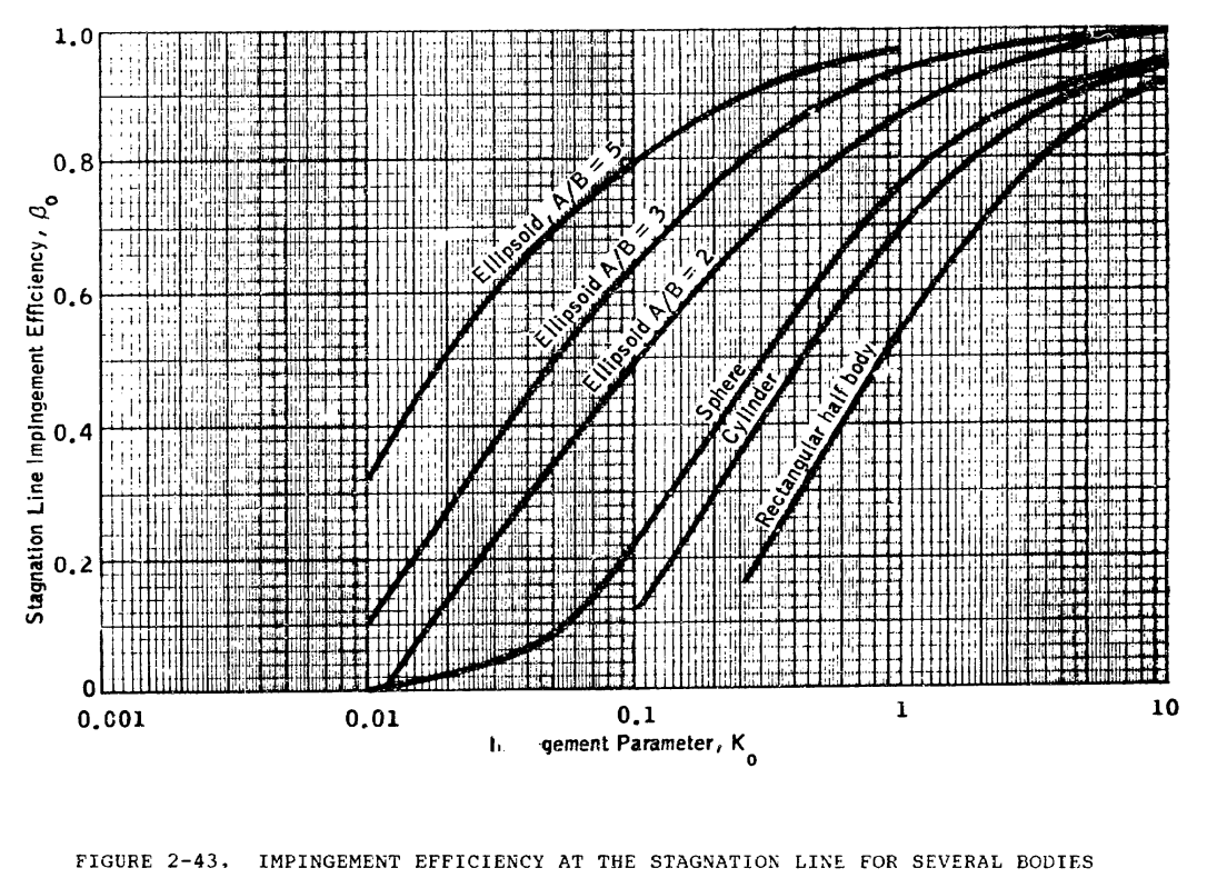
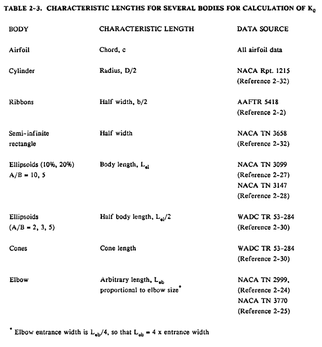
Note that the characteristic length used to calculate Ko is the cylinder radius or diameter / 2.
Equations 2-6, and 2-8 are used to calculate Ko.


Note that equation 2-10 could also be used.

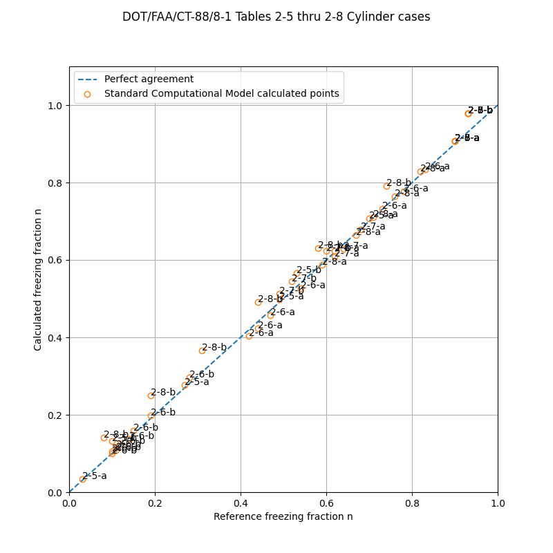
For the freezing fraction values, the comparison is "good", but the results from Table 2-8b (having higher airspeeds) have an offset. The handbook values are "reference", and the values calculated with the python program are "calculated":
Public domain image by Donald Cook.
The percentages of the heat sources and sinks are similar, but not identical, to the values listed in the handbook ("reference"). Some cases, like 2-5-b at -2C, have some differences greater than 10%, but the freezing fractions were similar (0.10\0.13).
DOT/FAA/CT-88/8-1 Tables 2-5 thru 2-8 cylinder cases
                   Reference\calculated
                              Heat Sources         Heat Sinks
Case   TC  V  MVD  n          %qv    %qf     %qk   %qc    %qe    %qw
2-5-a -26  70  20  0.90\0.91   5\ 4  94\95   1\ 1  48\49  16\16  36\34
2-5-a -20  70  20  0.70\0.71   6\ 5  93\94   1\ 1  47\48  18\18  35\33
2-5-a -14  70  20  0.49\0.50   8\ 7  91\92   1\ 1  46\47  21\21  33\32
2-5-a  -8  70  20  0.27\0.28  14\12  84\86   2\ 2  44\45  24\24  32\31
2-5-a  -2  70  20  0.03\0.03  53\48  38\43   9\ 9  44\46  25\23  31\32
2-5-b  -6  70  20  0.93\0.98  24\21  75\78   1\ 1  60\61  34\33   6\ 6
2-5-b  -4  70  20  0.53\0.57  36\32  63\68   1\ 1  59\61  35\33   6\ 6
2-5-b  -2  70  20  0.10\0.13  73\65  25\33   2\ 2  60\63  34\31   6\ 6
2-6-a -26  70  20  0.90\0.91   5\ 4  95\95   1\ 1  48\49  15\16  36\34
2-6-a -26  70  20  0.83\0.83   4\ 4  95\95   1\ 1  46\47  14\15  40\37
2-6-a -26  70  20  0.78\0.78   4\ 4  95\95   1\ 1  44\45  14\15  42\40
2-6-a -26  70  20  0.73\0.73   4\ 3  95\96   1\ 1  42\43  13\14  45\43
2-6-a -26  70  20  0.54\0.53   3\ 2  96\96   1\ 1  29\30   9\10  62\60
2-6-a -26  70  20  0.47\0.46   2\ 2  96\97   2\ 2  22\23   7\ 8  71\69
2-6-a -26  70  20  0.44\0.42   2\ 2  97\97   2\ 2  18\19   6\ 6  77\75
2-6-a -26  70  20  0.42\0.40   1\ 1  97\97   2\ 2  15\16   5\ 5  80\79
2-6-b  -6  70  20  0.93\0.98  24\21  75\78   1\ 1  60\61  34\33   6\ 6
2-6-b  -6  70  20  0.28\0.30  21\18  77\80   2\ 2  51\52  29\28  21\20
2-6-b  -6  70  20  0.19\0.20  18\15  79\81   3\ 3  44\45  25\24  32\31
2-6-b  -6  70  20  0.15\0.16  16\14  80\83   4\ 4  39\39  22\21  40\39
2-6-b  -6  70  20  0.14\0.14  14\12  82\83   4\ 4  34\35  19\19  46\46
2-6-b  -6  70  20  0.12\0.13  13\11  82\84   5\ 5  31\32  18\17  51\51
2-6-b  -6  70  20  0.11\0.12  12\10  83\85   5\ 5  28\29  16\16  56\55
2-6-b  -6  70  20  0.11\0.11  11\ 9  84\85   6\ 6  26\27  15\15  59\59
2-6-b  -6  70  20  0.10\0.10  10\ 9  84\85   6\ 6  24\25  14\13  62\62
2-6-b  -6  70  20  0.10\0.10   9\ 8  85\86   6\ 6  23\23  13\13  65\64
2-7-a -26  70  20  0.90\0.91   5\ 4  95\95   1\ 1  48\49  15\16  36\34
2-7-a -26  70  40  0.68\0.68   4\ 3  95\96   1\ 1  39\41  12\13  48\46
2-7-a -26  70  60  0.64\0.63   3\ 3  95\96   1\ 1  37\38  11\12  52\50
2-7-a -26  70  80  0.62\0.61   3\ 3  96\96   1\ 1  35\36  11\12  54\52
2-7-b  -6  70  20  0.93\0.98  24\21  75\78   1\ 1  60\61  34\33   6\ 6
2-7-b  -6  70  40  0.60\0.62  24\20  76\79   1\ 1  58\59  33\32  10\10
2-7-b  -6  70  60  0.52\0.55  23\20  76\79   1\ 1  57\58  32\31  11\11
2-7-b  -6  70  80  0.49\0.51  23\20  76\79   1\ 1  56\57  32\31  12\12
2-8-a -26  70  20  0.90\0.91   5\ 4  95\95   1\ 1  48\49  15\16  36\34
2-8-a -26  80  20  0.82\0.83   6\ 5  93\94   1\ 1  46\48  14\15  39\37
2-8-a -26  90  20  0.76\0.76   7\ 6  92\92   1\ 1  45\46  14\14  42\40
2-8-a -26 100  20  0.71\0.71   8\ 7  90\91   2\ 2  43\44  13\14  44\42
2-8-a -26 110  20  0.67\0.66  10\ 9  88\89   2\ 2  42\43  13\13  46\44
2-8-a -26 120  20  0.62\0.62  11\10  86\87   3\ 3  40\42  12\12  48\46
2-8-a -26 130  20  0.59\0.59  13\11  84\85   4\ 4  39\41  11\12  49\48
2-8-b  -6  70  20  0.93\0.98  24\21  75\78   1\ 1  60\61  34\33   6\ 6
2-8-b  -6  80  20  0.74\0.79  32\28  67\71   1\ 1  60\61  33\32   7\ 7
2-8-b  -6  90  20  0.58\0.63  40\35  58\64   1\ 1  60\61  32\31   8\ 8
2-8-b  -6 100  20  0.44\0.49  50\44  48\54   2\ 2  60\62  32\30   8\ 8
2-8-b  -6 110  20  0.31\0.37  61\54  37\44   2\ 2  60\63  30\28   9\ 9
2-8-b  -6 120  20  0.19\0.25  72\64  25\33   3\ 3  60\63  30\27  10\10
2-8-b  -6 130  20  0.08\0.14  85\76  11\20   3\ 4  61\64  29\25  10\11
I also ran this with a Langmuir D distribution (not shown). The results were very similar.
Aircraft Icing Handbook Figure 2-81
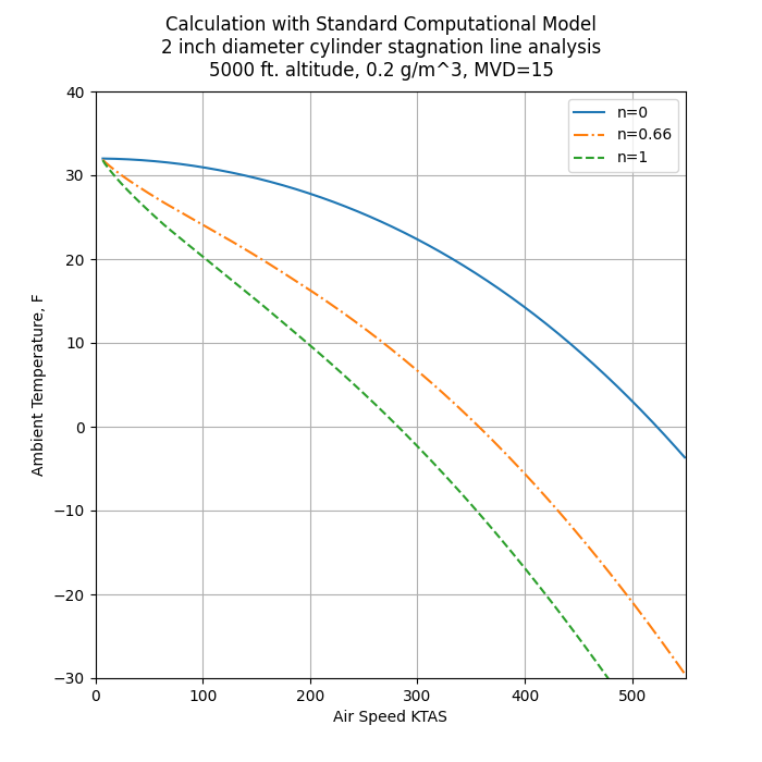
Figure 2-81 (and 2-82) show calculated cylinder stagnation line freezing fraction related to ice type: glaze 0 < n < 0.66, intermediate 0.66 < n < 1, rime n = 1.
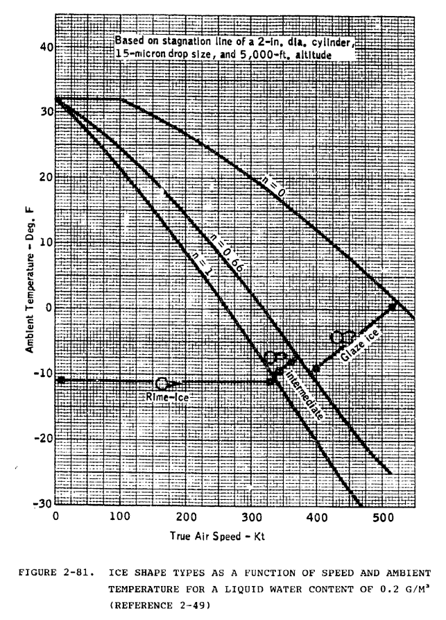
The Python implementation of the Standard Computational Model was also used to reproduce Figure 2-81 (file "intermediate/figure_2_81.py").
The method of determining the leading edge stagnation line water catch β value is not defined in the handbook text. For the calculations here, the cylinder line from Figure 2-43 is used.
A Langmuir A drop size distribution was assumed. The values are similar, but not identical, to Figure 2-81.
Public domain image by Donald Cook.
Conclusions
I view this as a representative implementation of the Standard Computational Model. However, after we have tried this example using LEWICE, there will be further discussion.
References (Handbook format)
2-2 Langmuir. I. and Blodgett, K., "A Mathematical Investigation of Water Droplet Trajectories," AAFTR 5418, February 1946. books.google.com
2-44 Analysis and Verification of the Icing Scaling Equations AEDC-TR-85-30 Vol. 1 (Revised)
2-45 Kreith, F., Principles of Heat Transfer, Intext Educational Publishers, New York, 1973, third edition archive.org [online borrowing with registration]
Related
Back to Intermediate Topics