Public domain image by Donald Cook.

Summary

Search within the Appendix C Continuous Maximum Icing definition for the thickest ice shape.

Prerequisites

You need to have completed Run a 2D simulation.

Introduction

"Aircraft Ice Protection" AC 20-73A faa.gov offers guidance on analysis for icing conditions. We will not cover the certification aspects in detail.

Much of the detail is on ice protection systems.

This advisory circular (AC) tells type certificate and supplemental type certificate applicants how to comply with the ice protection requirements of Title 14 of the Code of Federal Regulations (14 CFR) parts 23, 25, 27, 29, 33, and 35.

However, it is also useful for analysing ice shapes on unprotected surfaces.

It is noted that:

Determination of critical ice shape configurations is not straightforward and may require engineering judgment.

SAE AIR5903, "Droplet Impingement and Ice Accretion Computer Codes" sae.org notes:

A balancing of accurate and conservative results may be necessary to achieve a design that is both cost‑effective and safe.

We will only cover areas that can guide us in determining ice shapes for unprotected surfaces (with 233 pages, there is much more information in AC 20-73A). Ice shapes on unprotected areas may be determined by test or analysis. We will cover analysis here.

It is suggested that you track your time and computing resources required to perform the simplified analysis outline below. This will give you data to estimate what is required for a more complete analysis.

Discussion

Critical ice shapes

The task is to determine the Critical Ice Shape ("worst case"):

R.4.1 Considerations for Critical Ice Shapes.

A critical ice shape may be defined as the aircraft surface ice shape (formed within icing conditions defined by 14 CFR parts 25, Appendix C or 29, Appendix C) that results in the most adverse effects for specific flight safety requirements. The critical ice shape may differ for different flight safety requirements. For example, the critical ice shape may differ for stall speed, climb, aircraft controllability, control surface movement, control forces, air data system performance, “artificial feel” adjustments, ingestion and structural damage from shed-ice. Engine thrust, engine control, and aeroelastic stability considerations may result in different critical ice shapes.

Critical ice shapes may vary with aircraft configuration and flight phase...

Determination of critical ice shape configurations is not straightforward and may require engineering judgment...

You may use experience from previous certifications of similar aircraft designs as guidance for determining the icing conditions that produce candidate critical ice shapes. Unprotected critical surface ice shapes should reflect the icing exposure time associated with the respective phase of flight. For the holding configuration, consider the 45-minute holding period...

(There is more, but this is adequate for our simplified illustration here.)

Addressing all aspects (effect on stall speed, climb, aircraft controllability, control surface movement, control forces, air data system performance, “artificial feel” adjustments, ingestion and structural damage from shed-ice) is a complex topic that will not be detailed here.

Verifying ice shapes

Ice shapes from analysis may create an illusion of precision. The values may be reported to many digits, but they do not always match test data well.

A detailed discussion of verifying ice shapes is an advanced level topic. Here, we will summarize the AC 20-73A discussion on the topic.

R.5.4 Drop Impingement and Ice Accretion Computer Codes and Other Analytical Methods.
Applicants may use verified computer codes and analytical methods to predict ice shapes. The predicted ice shape is the result of calculations that define the flowfield, the drop trajectories, water loading, and the ice accretion physics. Many icing codes are available. They differ to varying degrees in their manner of modeling the ice accretion process. SAE ARP5903 (Reference R20) provides information that describes several available drop impingement and ice accretion codes.

Confidence in 2D icing codes to predict ice shapes accurately is mixed when their results are compared with icing wind tunnel ice. Figures R-21 through R-24 show reasons for this mixed confidence. The figures compare ice shapes predicted by several icing codes with those produced in two icing wind tunnels. The data from Reference R21 show that even at colder, rime ice conditions, where confidence in predicted ice shapes is highest, there are significant differences between predicted and empirical ice shapes.

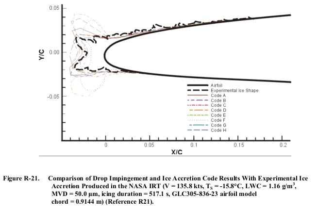
There is also variation in experimental ice shapes in repeated tests, but the variation is generally less than the variation in results from different codes.

Ice accretion codes with 3D flow field and drop trajectory abilities, coupled to a 2D ice accretion calculation, have been developed to predict 3D ice shapes. The experimental ice shape data available for verifying these pseudo 3D ice accretion codes is limited. Therefore, confidence in these ice accretion codes is limited. Also, none of the codes predict the periodic “scalloped” or “lobster tail” ice shapes that develop from ice feathers on swept wings.

For several recent ice shape comparison examples, including 3D codes, see "AIAA 1st Ice Prediction Workshop Results post-processing for code-to-code comparison" folk.ntnu.no. [Frankly, the level of agreement has not changed much in 16 years.]

Simplifications for a tractable analysis

We will simplify the task by assuming that the thickest ice shape has the greatest effect.

For ice protection, some analysis points are suggested. We will use them for determining ice shapes.

Table 6 shows the meteorological conditions you should consider for a typical compliance analysis for operating in continuous and intermittent maximum icing conditions.

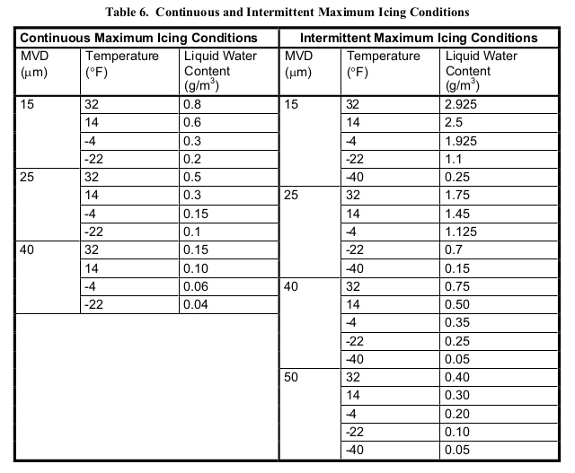
Here are the Continuous Maximum Icing Conditions values:

MVD micrometer	T F	LWC g/m^3
15	32	0.8
15	14	0.6
15	-4	0.3
15	-22	0.2
25	32	0.5
25	14	0.3
25	-4	0.15
25	-22	0.1
40	32	0.15
40	14	0.1
40	-4	0.06
40	-22	0.04

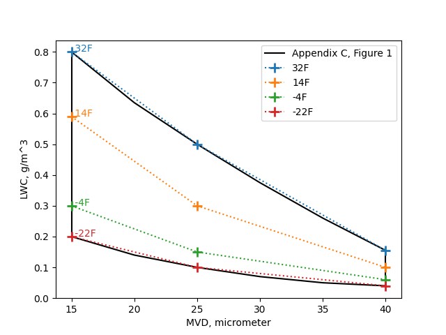
The selected points plotted on Appendix C Figure 1 are:

Public domain image by Donald Cook.

Select pressure altitudes that cover the range of altitudes associated with each temperature from figures E-2 and E-5 in appendix E of this AC.

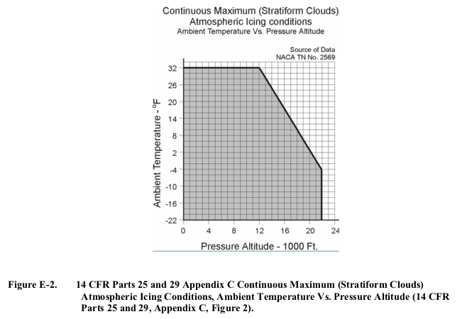
We will select the labeled altitude values that are within the range of the figure (0, 4000, 8000, 12000, 16000, and 20000 ft). Note, for example, that values at 32°F extend from 0 to 12000 ft, so values at 16000 and 20000 ft would not be applicable.

You should perform a [water] drop impingement and water catch analysis to evaluate the impingement limits and water collection characteristics of aircraft surfaces and components. This analysis also provides the ice collection efficiencies of aircraft surfaces and components. The analysis should consider all the airplane’s flight configurations, phases of flight, and operating envelopes (including airspeeds, aircraft configurations, and angles of attack).

We will consider only one flight phase here, nominally holding. We will only analyze one angle of attack (4 degrees).

For airspeed, we will assume a constant Equivalent Airspeed (EAS) value of 100 m/s (about 194 KEAS), with differing altitude and temperature combinations resulting in different true airspeed values. This maintains a constant dynamic pressure, so a nearly constant lift value is achieved at a constant angle of attack (with small variations for Mach and Reynolds number effects). See "Equivalent airspeed" wikipedia.org for more information on EAS.

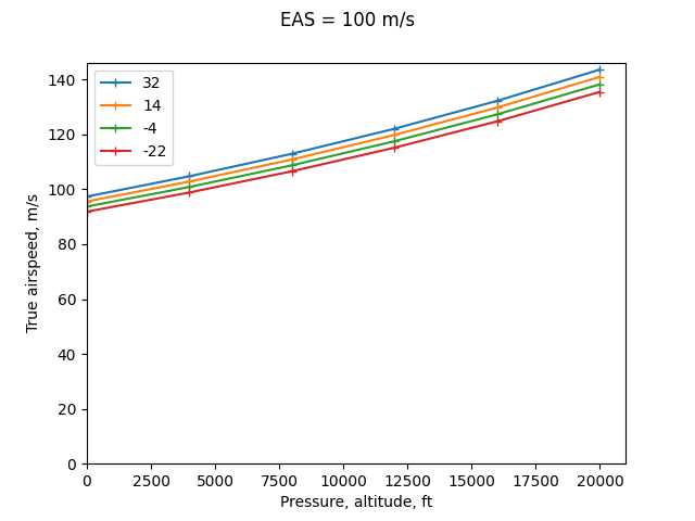
Public domain image by Donald Cook.

We will use a NACA0012 airfoil, with a chord length of 5 m. This does not represent a particular airplane, and is typical of Part 25 transports (some are larger and some are smaller, with respect to mean aerodynamic chord).

We will separately analyze the three MVD values for the combinations of altitude and temperature, and determine the maximum ice thickness at each point.

Analysis with LEWICE

This analysis will use the LEWICE code. As this is a 2D code, it does not take into account airplane level flow that can affect the local flow at a particular wing span location. The assumption that local 2D "effective" angle of attack equals the nominal angle of attack can be very approximate. A more thorough practice when the stagnation location is known (by wind tunnel tests or 3D analysis) is to vary the local 2D angle of attack to match the 3D flow stagnation line location.

See, for example, the AIAA Ice Prediction Workshop presentation "Boeing LEWICE2D and LEWICE3D summaries" folk.ntnu.no.

We will assume that the wing is not swept.

LEWICE does not have a direct way to account for sweep, but approximations have been used for swept wing cases. LEWICE also does not have a direct way of changing the ice density use (917 kg/m^3). If calibration data is available for a given configuration, a different ice density can give more accurate ice thickness values. An ice density of 917 kg/m^3 was used here.

A Langmuir D drops size distribution was used.

Here are example results with an MVD value of 25 micrometers:

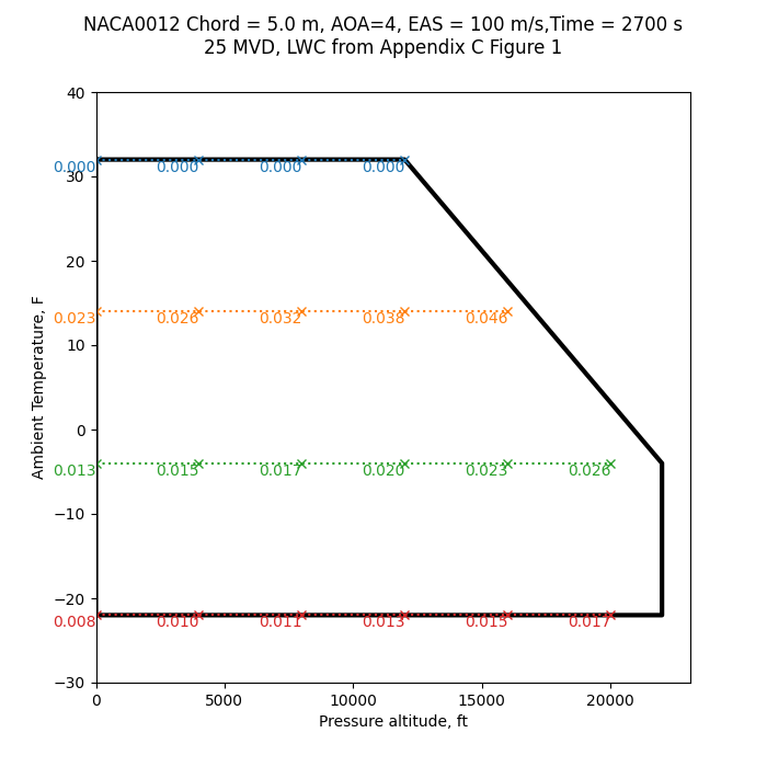
Public domain image by Donald Cook.

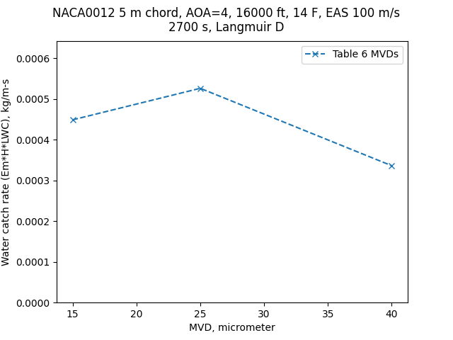
Selecting the altitude and temperature that yields the thickest ice (16000 ft, 14°F), we can do a sensitivity check on the effect of MVD:

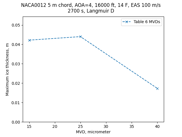
Public domain image by Donald Cook.

This may seem counter-intuitive, given that the highest liquid water content values occur at the smallest drop sizes. However, there is a complex interplay of several factors. The collection efficiency varies with drop size, which is one of important the factors. The total water catch (proportional to Em * LWC) can reach a maximum at an intermediate drop size:

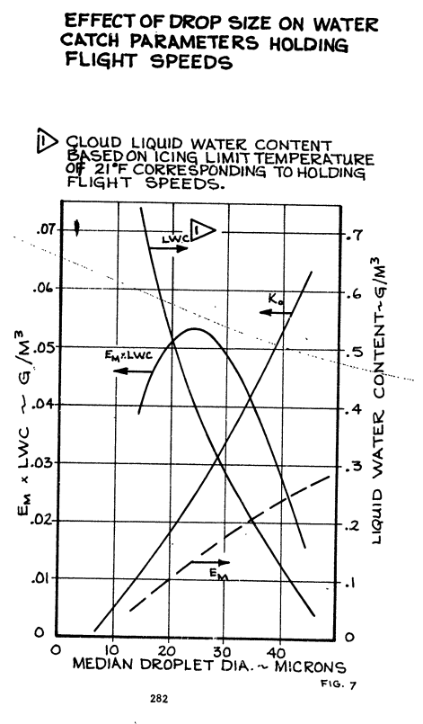
from "Aircraft Ice Protection Report of Symposium" apps.dtic.mil

Public domain image by Donald Cook.

However, different chord lengths and flight conditions will yield different results (do not assume that 25 micrometers will necessarily yield maximum ice thickness for your conditions).

A more detailed analysis

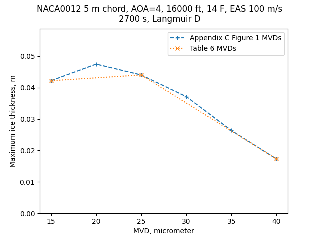
The steps between conditions in Table 6 may be considered to be large, so here the analysis is repeated with finer resolution to show the effect.

If we calculate the effect of MVD with the labeled values from Appendix C Figure 1 (with 5 micrometer increments rather than the 10 to 15 micrometer increments from Table 6), a peak ice thickness occurs at 20 micrometers, rather than the 25 micrometers from the Table 6 analysis points.

Public domain image by Donald Cook.

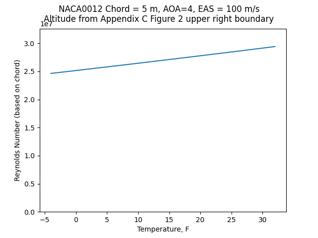
One can use insight from the analysis above to determine where to concentrate a search for thickest ice. In the figure where the Figure 1 envelope was over-laid with calculated ice thickness values, the thickness values generally increase as altitude is increased. So, it is apparent that there will be a maximum along the upper-right boundary of Appendix C Figure 1. We will search that in 2°F increments (resulting in about 440 ft. altitude increments).

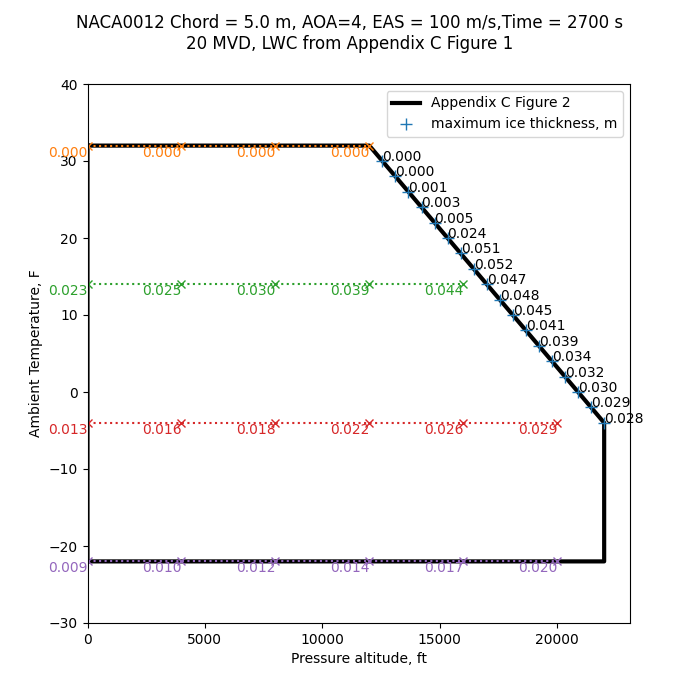
Public domain image by Donald Cook.

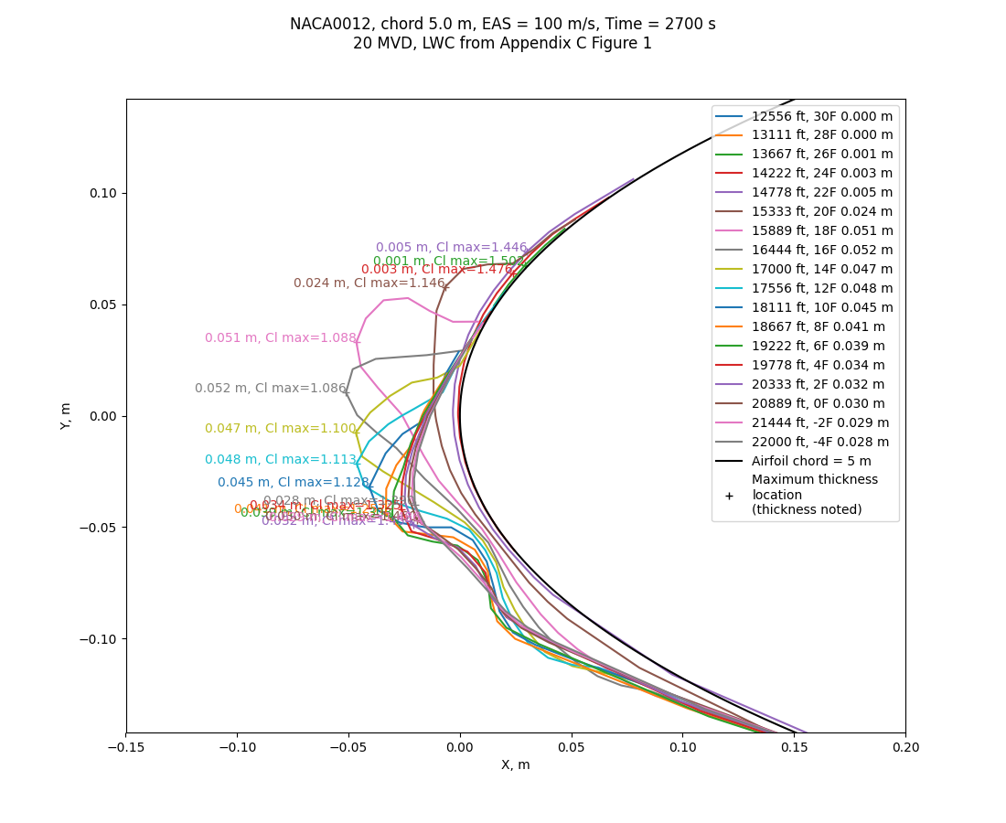
The analysis yields a series of ice shapes:

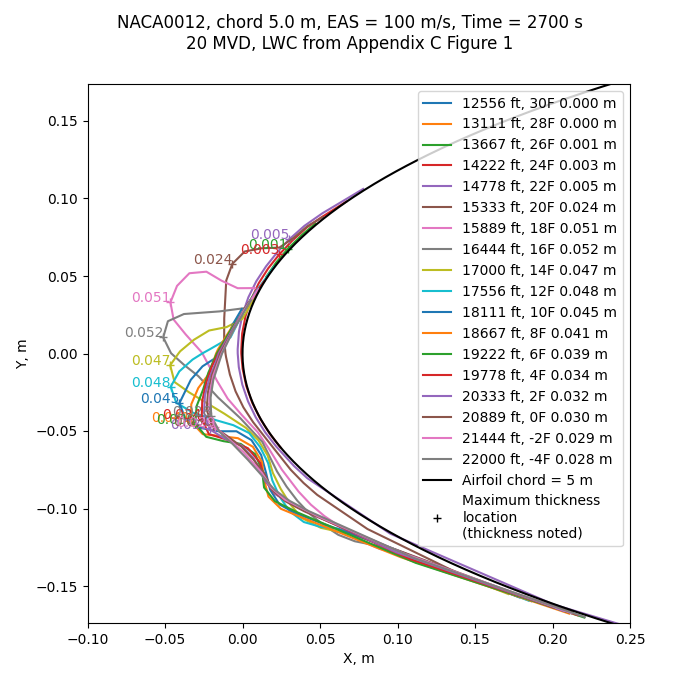
Public domain image by Donald Cook.

The case ice with the thickest ice was at 16°F. However, the case at 18°F was nearly as thick.

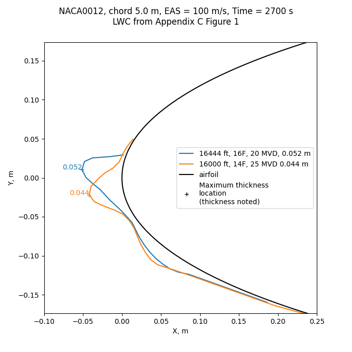
The thickest ice (0.052 m at 20 MVD) is greater than that from the sparser search (0.044 m at 25 MVD).

Public domain image by Donald Cook.

At a full-scale view, the ice shapes are barely discernible, and the differences even less so:

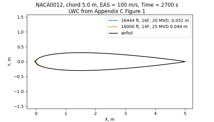
Public domain image by Donald Cook.

I view the difference between the two ice shapes to be large enough to merit the finer resolution search. However, quantifying that difference for all aspects such as "stall speed, climb, aircraft controllability, control surface movement, control forces, air data system performance, “artificial feel” adjustments, ingestion and structural damage from shed-ice" is quite challenging, and is not detailed here.

Effect on Cl_max

We will estimate the effects on Cl_max. For this example, the Reynolds number values are close to that of available data (RE 3.1e7) for a protuberance that we saw in Introduction to Variations:

Public domain image by Donald Cook.

We can add the estimated Cl_max value onto the ice shape figure (20 MVD case shown):

Public domain image by Donald Cook.

We will concentrate on the range of temperatures with the minimum Cl_max values. For each drop size considered, the effect has a minimum value of Cl_max at some ambient temperature of between 16 and 20 F. The overall minimum is at MVD = 20 and 16 F, as we saw above, but there are several combinations that have Cl_max ~= 1.10, that may well be considered "close enough", especially given that much interpolation within widely spaced data was required to estimate the effect.

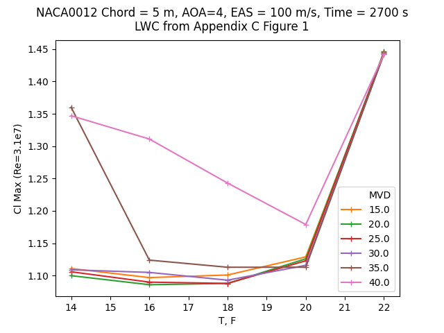
Public domain image by Donald Cook.

However, for other conditions and airfoils the maximum effect may well be at some other temperature and drop size.

For these cases, the largest effect corresponded to the thickest ice shape. However, that may not hold for all cases, particularly for smaller chord lengths, where the relative position of ice horns can be further back on the airfoil.

Exercises

Consider an analysis for Intermittent Maximum Icing conditions (Appendix C figures 4, 5, and 6). What time exposure do you select?

Repeat the analysis, assuming that the Appendix C Figure 3 Liquid Water Content Factor is applicable (AC 20-73A 8.2.2.6(c) refers to the Liquid Water Content Factor as "a horizontal extent correction"). Did the critical condition change?

Resources

"Aircraft Ice Protection" AC 20-73A faa.gov

Related

Back to Intermediate Topics