From AC 20-73A faa.gov.
Summary
- Different methods (test, analysis methods) can yield different ice shapes for the same conditions
- Measurements of ice shape parameters characterize the differences
- What is "too large" of a difference depends on unique factors for a particular case
- Engineering judgment is required to navigate the differences
Discussion
A method to characterize ice shapes
"Aircraft Ice Protection" AC 20-73A faa.gov lists ice shape parameters that can be used to compare ice shapes:
Applicants may use the lists of ice shape and water catch evaluation parameters in tables R-1 and R-2, ranked against their adverse airplane effects, to compare simulated and natural ice shapes. These lists are from SAE ARP5903 (Reference R20).
Table R-1. Ranking of Ice Shape Evaluation Parameters
| Rank | Parameter | Units | Conservatism criteria |
|---|---|---|---|
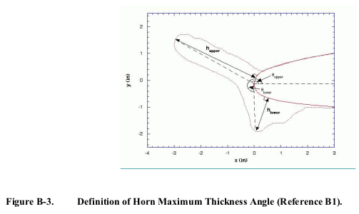
| 1 | Upper (suction surface) horn height | Equal or greater horn peak thickness (height) | |
| 2 | Upper Horn Angle | degree | Criticality of location (at upper peak thickness) |
| 3 | Lower (pressure surface) height | Equal or greater horn peak thickness (height) | |
| 4 | Lower Horn Angle | degree | Criticality of location (at lower max. thickness) |
| 5 | Total ice cross-sectional area | Equal or greater area | |
| 6 | Leading edge minimum thickness | Equal or smaller thickness | |
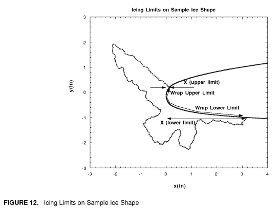
| 7 | Upper accretion limit | % x/c* | Equal or greater x/c |
| 8 | Lower accretion limit | % x/c* | Equal or greater x/c |
NOTE: The first four parameters assume that icing horns exist. This is not always the case.
* Percent of local component chord
SAE ARP5903 "Droplet Impingement and Ice Accretion Computer Codes" (Reference R20) is available at sae.org.
Accretion limits are defined:
"Horns" are defined:
Differences in ice shapes between test and analysis
The most detailed comparison data to date is NASA/TM-2008-215174 nrts.nasa.gov.
Figure 7 shows the comparison for the lower and upper ice horns while figure 8 shows the comparison for lower and upper horn angle. The comparison of SLD shapes to experiment shows approximately the same difference as for standard ice shapes. For the experimental ice shapes, the upper and lower horns were selected manually rather than allowing THICK to automatically select the largest feature. This process was used due to the high variability of the experimental ice shapes. THICK often has trouble locating the correct horn locations without manual intervention. Running THICK automatically on each shape produced the code values for horn thickness and horn angle. This was done to save time in the analysis and was justified on the basis that the code results are smoother and an automated process could be used. However, it is possible that THICK did not select the correct horn locations for all cases.
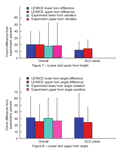
I read the differences as 20% for upper height and 26 degrees for upper horn angle.
LEWICE (2D) is the only code that I know of that has been characterized to this level of detail.
Note that the characterization method and data are largely for two-dimensional geometries. While detail-rich, 3D scans have been made of ice shapes, including scalloped horns on swept wings, general characterizations of 3D geometries have not yet been well-developed.
Variations in analysis methods
AC 20-73A:
R.5.4 Drop Impingement and Ice Accretion Computer Codes and Other Analytical Methods.
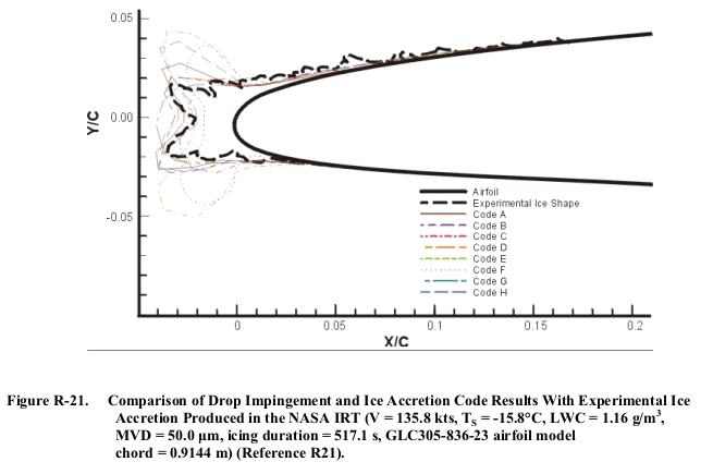
Applicants may use verified computer codes and analytical methods to predict ice shapes. The predicted ice shape is the result of calculations that define the flowfield, the drop trajectories, water loading, and the ice accretion physics. Many icing codes are available. They differ to varying degrees in their manner of modeling the ice accretion process. SAE ARP5903 (Reference R20) provides information that describes several available drop impingement and ice accretion codes.Confidence in 2D icing codes to predict ice shapes accurately is mixed when their results are compared with icing wind tunnel ice. Figures R-21 through R-24 show reasons for this mixed confidence. The figures compare ice shapes predicted by several icing codes with those produced in two icing wind tunnels. The data from Reference R21 show that even at colder, rime ice conditions, where confidence in predicted ice shapes is highest, there are significant differences between predicted and empirical ice shapes.
While the results from the codes differ from one another and from the test ice shape, at least some may be viewed as "conservative" (if not particularly accurate), in that the horn thickness determined by analysis is greater than that from test. Several of the codes have purportedly been used for certification work.
Reasons why ice shapes produced by various icing wind tunnels, computer codes, and other analytical methods may vary include:
- Calibration of the icing wind tunnel.
- The uniformity and qualities of the tunnel’s flow and icing cloud.
- Other tunnel testing considerations.Reasons why ice shapes produced by various ice accretion computer codes, and other analytical methods, vary include:
- Differing algorithms and assumptions used in the computer codes and analytical methods.
- The use of various computer code versions and inputs.
- The use of empirical ice shapes from different sources to “tune” computer codes and other analytical methods (to account for unknown icing physics and other effects).
For several recent ice shape comparison examples, including 3D codes (and the codes identified), see "AIAA 1st Ice Prediction Workshop Results post-processing for code-to-code comparison" folk.ntnu.no. The differences between codes have not reduced much since AC 20-73A was published in 2008.
Trends of ice shape effects
Some general studies of ice shape effects have been published. These have been largely for 2D geometries. They have also generally been at lower Reynolds number values, and Reynolds effects can influence results.
The effects are unique for each airfoil. On an airplane level, where many wings have sweep, twist, and taper, results can be configuration specific, and the general correlations do not take those into account. Results can be sensitive to the Reynolds and Mach number values. These and other factors limit the general applicability of using these data to other airfoils and flight conditions.
While the general data may not give accurate absolute values, they have been used to inform engineering judgment to identify among many possible candidates the ice shape most likely to have the largest effects.
Some studies have placed protuberances on the airfoil, and measured the effects. This may relate well to the effect of an upper surface ice horn.
AC 20-73A:
R.4.2 Aerodynamic Considerations for Determining Critical Ice Shapes.
...
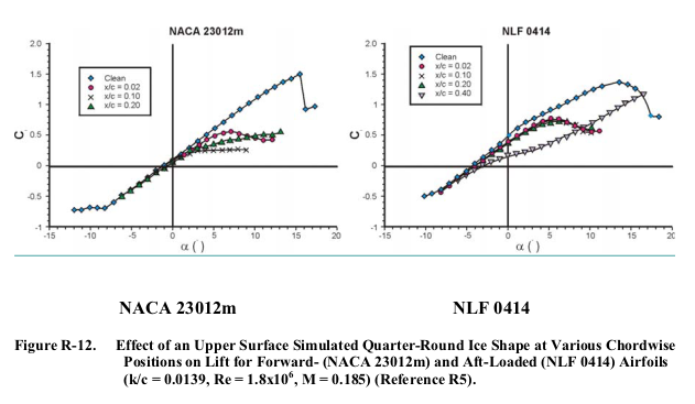
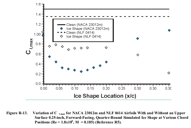
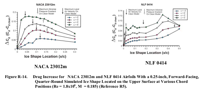
Figure R-12 shows low Reynolds number wind tunnel test results. These data resulted from installing a 1⁄4-inch simulated ice shape (quarter-round) at various chordwise locations on 18-inch models of each airfoil. Figure R-13 shows the maximum lift values. Although these aerodynamic characteristics are Reynolds number dependent, the data show where the ice builds up is important and show the influences of the ice buildup on the behavior of the boundary layer and the airfoil aerodynamic performance.
The examples in AC 20-73A were for a fixed protuberance height (0.25 inch) The cited reference R5, DOT/FAA/AR-00-14 "Effects of Large-Droplet Ice Accretion on Airfoil and Wing Aerodynamics and Control" faa.gov considered other heights and found that:
Aerodynamic penalties became more sever[e] as the height-to-chord ratio of the simulated ice shape was increased from .0056 to .0139.
The data appears to support that an ice "horn" can be approximated as a protuberance, as the shape of the protuberance had only minor effects:
The variation in the simulated ice shape geometry had only minor effects on the airfoil aerodynamics.
Other data also show that the height of a protuberance (H/C) as well as location can affect performance. "Airfoil Section Characteristics as Affected by Protuberances" NACA-TR-446, ntrs.nasa.gov shows trends with height that can be non-linear, and are dependent on position for the NACA0012 airfoil:
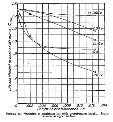
From NACA-TR-446.
For larger airfoils, all of the ice may be in the first few percent of X/C, and any "horns" farther forward, virtually at X/C=0 (for the base of the horn). So, in the figure above, the effect on lift may increase with height up to a point for X/C near zero, but had little increase for H/C > 0.005.
See the blog post "Conclusions of the Ice Shapes and Their Effects Thread" for several other examples of general correlations.
Relating LEWICE variations to effects on lift
We can compare the effect on lift noted in NACA-TR-446 of protuberances on a NACA0012 airfoil with the average difference of calculated upper horn location and thickness for LEWICE calculations compared to test values.
We will use the thickest protuberance in NACA-TR-446, H/C = 0.0125, as this is the easiest to see when plotted.
The values from the figure above are mapped around the airfoil in fairly small increments of Cl max value. Linear interpolation was used.
The tested protuberance locations are shown, and a LEWICE upper horn tolerance box drawn around that "horn". The LEWICE angular position tolerance is +/- 26 degrees (average difference from experiment), so the size of the tolerance box varies with distance from the center of curvature. It was also assumed that the maximum ice thickness equals the potential accumulation (equation 3 of NASA/CR-1999-208690), which determines the ice height tolerance (+/- 20% of the potential accumulation).
The actual ice horn height is typically less than the potential accumulation (but can also be greater), so the height tolerance depicted is not accurate for all cases; it is intended as an order-of-magnitude illustration only.
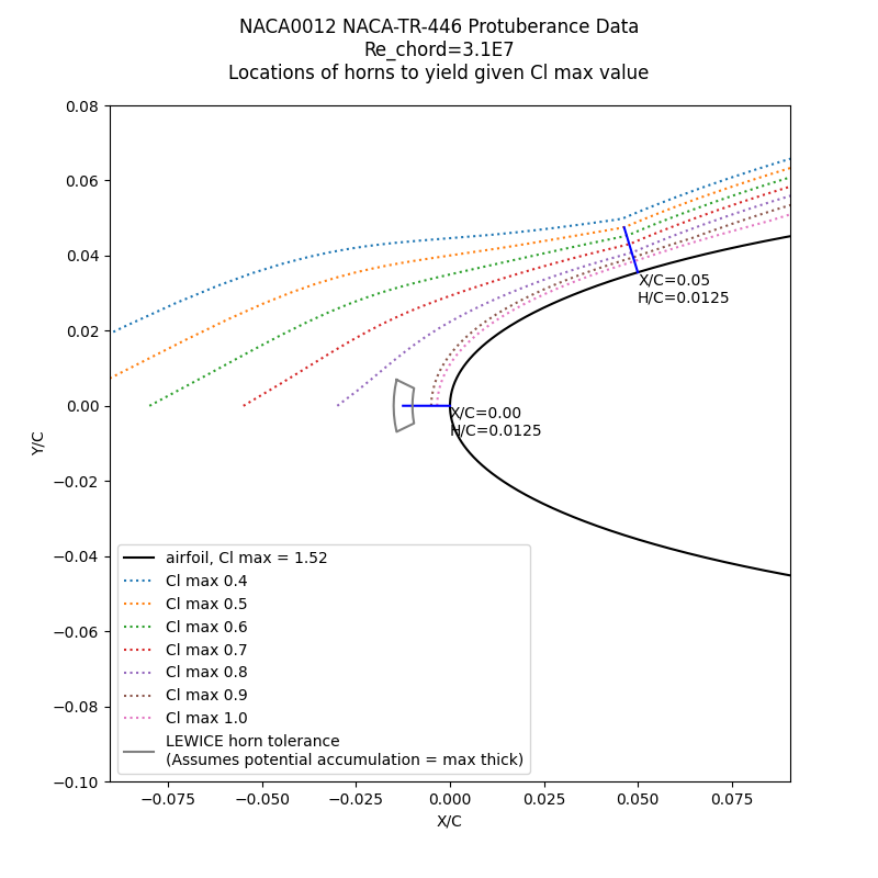
Public Domain image by Donald Cook.
For the protuberance at the X/C = 0 location, neither the location nor the thickness tolerance would have a large effect, with the interpolated Cl values close to the nominal 0.87.
The data from DOT/FAA/AR-00-14 for the effect of protuberances on the 23102m airfoil is further described in Lee, 2001 icing.ae.illinois.edu. We can use that data to make a plot similar to that for the NACA0012 airfoil.
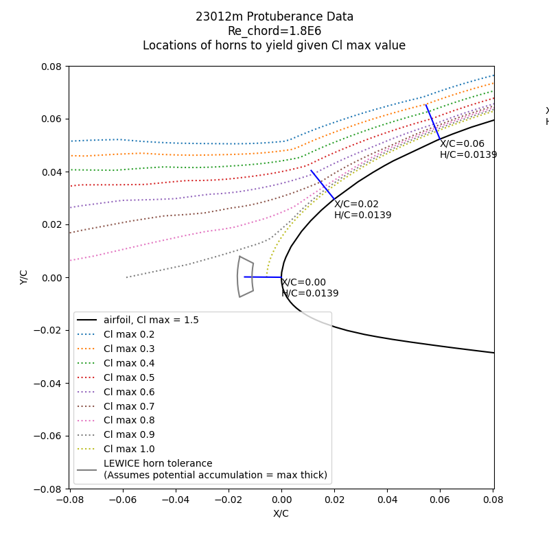
Public Domain image by Donald Cook.
I did not find a detailed enough data source for the effect on other airfoils to do more comparisons.
What is a "large" difference in ice shape?
The answer to the question of what is a "large" difference in ice shape depends on the situation.
One way to address the question is how close you need to be to a performance parameter, such as Cl max. If you want to know the effect, for example, to within +/- 5%, 2%, or whatever, and you have rich enough data to make a plot such as above, you can determine an allowed ice shape tolerance. For LEWICE, you can compare that to the expected shape differences.
There are other performance parameters (drag, moment, etc.) of interest that may be different from the lift trends noted above.
For other tools, I have not seen the variations as well-defined as for LEWICE.
Related
Back to Intermediate Topics