Public domain image by Donald Cook.
Prerequisites
You need to have completed Anti-Ice Heating Calculations Theory.
Introduction
For this we will use "Engineering Summary of Airframe Icing Technical Data", ADS-4, as the anti-ice examples are more detailed than those in the "Aircraft Icing Handbook", DOT/FAA/CT-88/8-1.
The ADS-4 analysis method uses NACA-TN-2799, from 1952, for the heat and mass balance calculations. This method implements solutions as nomographs (for more details, see the post NACA-TN-2799). We will not be using the nomographs. The heat balance equations are similar to the Standard Computational Model, which we will use.
The calculations are implemented in the file "aircraft_a_ads4.py" (and associated files) available at github.com/icinganalysis/icinganalysis.github.io. Readers are encouraged to run the analysis to the duplicate results.
Discussion
"Aircraft Icing", AC 20-73A, briefly mentions the terms Qa and Qr:
Qa Heat available
Qr Heat required
Heat required is the heat that leaves the surface needed to provide ice protection. Heat available is heat that leaves the heat surface that is available for anti-ice protection. Another term is heat supplied, the heat energy that an ice protection system consumes. Not all of the heat supplied may reach the outer heated surface where it is useful for ice protection.
System thermal efficiency is defined:
efficiency = (heat available) / (heat supplied)
The discussion below centers on the heat required. The other terms will not be detailed here.
Anti-ice heating
The "TYPICAL TWIN-ENGINE LIGHT PLANE A" example is particularly detailed, even though
hot gas [anti-ice] systems are not generally suitable for light aircraft and are not likely to be used because of their high weights and costly installation
4.1.4
4.1.4.1
STUDY OF VARIOUS ICE PROTECTION SYSTEMS FOR A TYPICAL TWIN-ENGINE LIGHT PLANE
SELECTION OF ICE PROTECTION FOR WING AND EMPENNAGE -
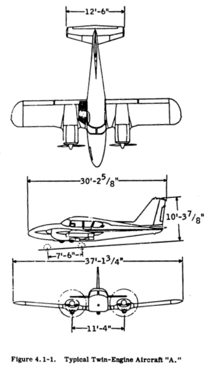
In selection of ice protection for light airplanes, the wings and empennage will be treated together since they would have the same type system. The water catch and impingement limits are calculated first to determine the extent protection is necessary. This is illustrated by the following sample calculations for the wing of twin-engine aircraft "A" shown in Figure 4.1-1:
Calculation of Impingement Limits and Water Catch
Wing - twin-engine aircraft "A"
Gross weight, 4,800 lb.
USA 35-B airfoil (12 per cent thick)
Wing area, A = 207 sq. ft.
Chord length, C = 67 in.
205 mph cruise at 7,000 ft. altitude (75 per cent power)
Ambient temperature, t = 17° F (most probable icing temperature from Figure 1-16)
Droplet diameter, Dd = 20 microns
Liquid water content, LWC = 0.46 gm/m3 (Figure 1-26)
Air density, pa 0.001996 slugs/cu.ft.
Air viscosity, p 0.36 x 10⁻⁸ slugs/ft.-sec.
Dynamic pressure, q = 90.2 psf (from page 4.1-9)
Lift coefficient, CL = 0.257 (from page 4.1-9)
The angle of attack can then be estimated from a CL versus a curve (Figure 4.1-2) for the given airfoil:
alpha = -1.7 [note: -1.6 is used below] Droplet Reynolds Number Re_d = 109 lambda/lambda_s = 0.342 (From Figure 2-6) Inertia parameter K = 0.0695 (This formula is equivalent to that of Section 2.)
Modified inertia parameter Ko = 0.0238
The ratio of projected airfoil height to chord h/C= 0.1225 (at alpha = -1.7), based on measured values for USA 35-B airfoil
Collection efficiency can be obtained from Figure 2-7 for a 12 per cent Joukowski airfoil at a zero-deg. angle of attack
EM = 0.135
Water catch WM = 2.95 lb/hr-ft.spanThe limits of impingement can be found from Figures 2-15 and 2-16 using a 15 per cent Joukowski airfoil at alpha = 2 deg. to represent the USA 35-B airfoil at alpha = -1.6 deg. The Joukowski airfoil was used because of the profile similarity to the USA 35-B airfoil for which no data was available. See Paragraph 2.3.4 for an explanation of airfoil matching procedures.
SU/C = 0.04 SL/C = 0.02
SU = 2.7 in. SL = 1.3 in.
(These values are not typical of other classes of airfoils; more commonly, impingement limits are greater on the lower surface.)
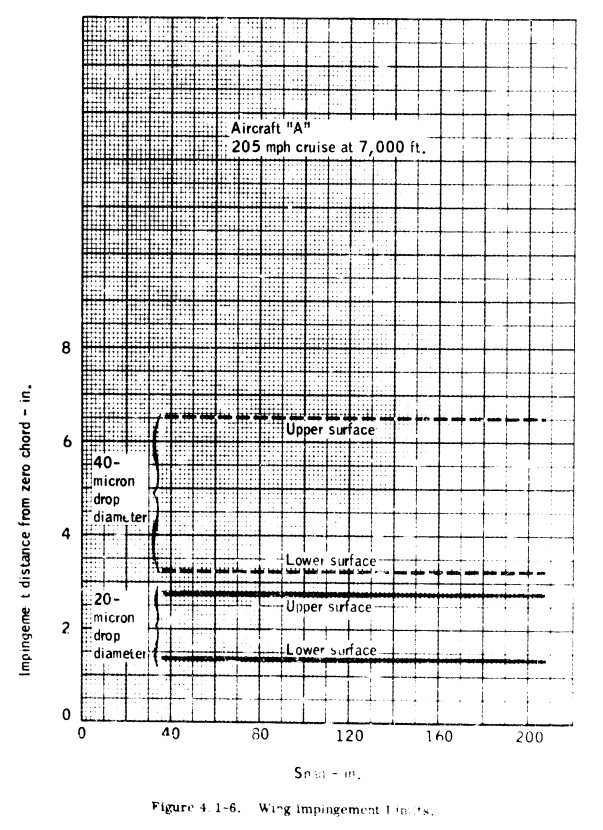
Figure 4.1-6 shows impingement limits versus span for the wing at both 20 and 40-micron drop sizes.
The determination of local water collection rate, Wb is illustrated for the wing of the same airplane by the following calculations:Calculation of Local Water Collection Rate
205 mph cruise at 7,000 ft. altitude Droplet diameter, Dd = 20 microns Liquid water content, LWC = 0.46 gm/m 3 (from Figure 1-26) Modified inertia parameter, Ko = 0.0238 (from above)
At the stagnation point, the local collection efficiency Beta = 0.46 (from NACA TN 3839, Ref. 4.1-4) using the 15 percent Joukowski airfoil at 2-deg. angle of attack to approximate the USA 35-B airfoil at -1.6 dog.
Local water collection rate, therefore, is:
Wb = 14.57 1b./hr.-sq.ft.
Values of local collection rate can also be found for different chordwise locations on the airfoil and, therefore, the local water found and plotted versus distance from zero chord as shown in Figure 4.1-9 for the wing. Curves for both 20 and 40-micron drop sizes are shown. The 40-micron curves shown in those figures are normally used to determine the necessary chordwise extent of ice protection. Although it in not necessary to protect entirely the 40-micron limits of impingement, protection is usually extended to between the 20 and 40-micron limits, where only a small amount of ice would remain beyond the protected area. For example, for this typical, twin-engine aircraft, it appears that ice protection should extend about six inches from zero chord on the upper surface and four inches on the lower surface of the wings, and about 2.6 [? last digit not clear], inches from zero chord on both surfaces of the horizontal stabilizer and vertical fin. The final choice of area protected is, of course, the prerogative of the designer and may depend on spar location and/or various other factors.Requirements for Hot Gas Anti-Icing
Hot gas anti-icing systems use several sources of hot gas. Direct exhaust-gas heat exchanger, combustion heater, and vapor cycle systems have been used (see Paragraph 3.5). However, hot gas systems are not generally suitable for light aircraft and are not likely to be used because of their high weights and costly installation. "Add-on" type systems are more desirable for light aircraft because they are less costly to install. Nevertheless, for completeness of this report, calculations of hot gas system heat and airflow requiremeents are illustrated below for the wing and tail of aircraft "A." Results are shown for both evaporative and running-wet systems; however, small aircraft anti-icing systems are seldom designed to be completely evaporative.Wing of typical light twin (Aircraft "A")
205 mph cruise at 7,000 ft. altitude
Ambient temperature, t = 20° F (conventional design point)
Ambient pressure, p = 23.1 in. Hg
Average surface heat transfer coefficient, h = 27.5 BTU/hr.-ft.2-F (determined graphically as described in Paragraph 3.5 and Figure 3-10)
Water catch, WM = 2.95 lb./hr.-ft. span (calculated above)
Average wrap-around distance = 15 in. (heated area extends to front spar - 10 per cent chord) Heated area/ft, span 1.25 sq.ft.
Water impingement rate, MW= 2.36 lb/hr-ft^2,
Using the method of NACA TN 2799 (Ref. 4. 1-5) described in Paragraph 3.5, for an evaporative system WM/ha = 0.0858
tau_4 = 11.3 F (from Figure 3-18)
t_s - t_o = 54.5 F
tau_3 = 102.7 F Therefore, t_s = 74.5 F (from Figure 3.18)
tau_1 = 59.5 F (from Figure 3.18)
tau_2 = 7 F (from Figure 3.18)
tau_5 = 0 F (assuming local static pressure equal to freestream pressure - Figure 3-18)
Surface heat requirements
Q = 3,960 BTU/hr.-ft.^2 (see Figure 4.1-13)
or 4,950 BTU/hr.-ft. span
or 89,000 BU/hr. (for 18 ft. of span)
The required anti-icing airflow can be estimated using the equation:W = Q / Cp (t_g - t_s) eta_c
in which the channel efficiency, eta_c, will normally be from 0.5 to 0.8 depending upon the chordwise channel length and on whether the system is a high or low-pressure system. A method for calculating the channel efficiency can be found in Appendix E of NACA TN 2866 (Ref. 4. 1-6).
Assume gas temperature, t_g = 350 F Specific heat of air at 350 F, Cp = 0.244 BTU/lb.-F The required anti-icing airflow for a low pressure system with a relatively short channel length (assuming eta_c = 0.5) would be:
w = 0.73 lbm/s
If the system were a high pressure system, the channel efficiency would be more like 0.8 and the anti-icing airflow required would be:w = 0.46 lb/sec.
(A channel efficiency of eta_c = 0.5 is probably the better assumption for light aircraft.)
Note that the surface wetness fraction K value is not mentioned; it is implicitly 1.
In ADS-4 section 2.3.2 it is noted:
Impingement limits are determined by the maximum droplet size in the cloud. Thus, for design purposes, 40 microns is often used to determine impingement limits, whereas 20 microns is often used to calculate water catch.
We calculate a surface wetness fraction K value based on the heated wrap distance of 15 inches and the 40 micrometer impingement limits (-3.3, 6.5 inches):
K = ((SU + SL) * 1 + 0.3 * (HEATED_WRAP - (SU + SL))) / HEATED_WRAP = 0.76
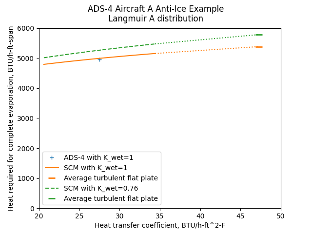
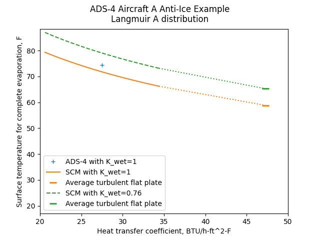
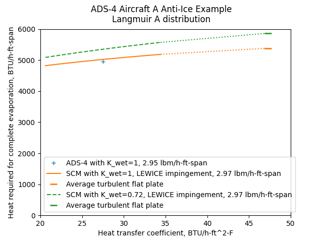
We will consider a heat transfer coefficient range of +/-25% about the nominal value of 27.5 BTU/h-ft^2-F, and calculate the heat required to evaporate all of the water using the Standard Computational Model. We will also consider using the turbulent flat plate method used in SAE AIR1168/4.
Public domain image by Donald Cook.
In the heat transfer coefficient range of +/-25% about the nominal value of 27.5 BTU/h-ft^2-F, the heating values vary by less than 25%. The heat transfer coefficient for the turbulent flat plate is notably higher than the nominal heat transfer coefficient.
For K = 1, the ADS-4 heating value and the SCM values agree well at the nominal heat transfer coefficient. With K = 0.76, the values are about 5% higher.
The heated surface temperature required to evaporate all of the water also varies some with the heat transfer coefficient and the K values.
Public domain image by Donald Cook.
If we use LEWICE to determine the impingement data, the values are slightly different. If you have access to LEWICE or another impingement calculation program then you are encouraged to perform the analysis. If not, values are provided (see USA 35-B Airfoil Impingement Data).
                      20 micrometer   40 micrometer
Method   LWC, g/m^3   Em              Sl, inch  Su, inch
ADS-4:   0.46         0.135           -3.30     6.50
LEWICE:  0.45         0.142           -2.09     6.83
The use of LEWICE impingement data has only a minor effect on the values:
Public domain image by Donald Cook.
Running wet heating
Requirements for Cyclic Electrical De-Icing
With cyclic electrical de-icing systems, continuously heated parting strips divide the ice buildup into portions which will shed more easily (with the help of aerodynamic forces) when power is applied to the cycled areas. Parting strips, which are normally one inch wide, should be laid out in a spanwise direction on the leading edge (at stagnation) when the sweep angle is less than 30 deg. Chordwise parting strips are used when the sweep angle is more than 30 deg. The protected area is divided into a number of smaller (cycled) areas which receive power alternately to minimize the total power required. A normal total cycled time is about three minutes. That is, each cycled area receives power once every three minutes. (See Paragraph 3.6.1.1 for more details on cyclic electrical de-icing systems.)Cycled area power requirements: Assuming a heat-on time of 20 sec. and t_o = 0° F, the datum temperature, t_ok is about 5° F (from Figure 3-8). The input power density then is approximately 12 watts/sq.in. from Figure 3-26, which was taken from NACA RM E51J30 (Ref. 4.1-7). An ambient temperature of 0° F was chosen as representative of the probable minimum icing temperature that would be encountered by a light aircraft operating at low altitude. Power requirements for a cyclic electric system are at a maximum at minimum ambient temperature (for a given airspeed). Parting strip power requirements for the wing of Aircraft "A":
205-mph cruise at 7,000 ft. altitude
Ambient temperature, t = 0 F (normal design point)
Liquid water content, LWC w 0.25 g/m3 (from Figure 1-26)
Modified Inertia parameter, Ko = 0.0238 (calculated previously)
Local collection efficiency at stagnation, Beta_max = 0.46 (calculated previously)
Local collection rate at stagnation therefore is:
WB = 0.329 (U) (LWC) Beta_max = 0.329 (205 mph)(0.25 g/m^3)(0.46)
=7.75 lb./,hr.-sq.ft.
Average surface heat transfer coefficient,
ha = 28.3 BTU/hr.-ft.^2-F (determined graphically as described in Paragraph 3.5)
Using the method of NACA TN 2799 (Ref. 4.1-5):
WM/ha = 7.75/28.3 = 0.274 Assuming the surface temperature, ts = 35° F, tau_1 through tau_5 can be found from Figure 3-18:
tau_1 45° F tau_2 7° F tau_3 24.5° F tau_4 4.5° F tau_5 0° F (assuming local static pressure equal to freestream pressure) Surface heat requirements Q= ha(tau_1-tau_2+tau_3-tau_4+tau_5) =(28.3 BTU/hr.-ft.^2-F)(45-1+24.5-4.5+0)
= 1,640 BTU/hr.-ft.^2
or 3.33 watts/sq. in.
Actual heater input power requirements will be approximately Q/0.6 or 5.5 watts/sq.in. assuming 60 per cent of the input heat would be transferred to the outer surface. The 60 per cent efficiency appears to be a good number based on previous experience (see NACA RM E51J30 - Ref. 4.1-7).
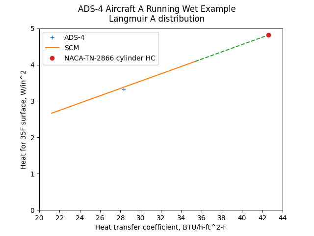
We will consider a heat transfer coefficient range of +/-25% about the nominal value of 27.5 BTU/h-ft^2-F. We will also consider the laminar cylinder approximation from section ADS-4 section 3.5.2 for the leading edge (see Anti-Ice Heating Calculations Theory).
Public domain image by Donald Cook.
As this case is at the stagnation line, the surface is fully wet.
The heating required is nearly directly proportional to the heat transfer coefficient. The heat transfer coefficient with the cylinder approximation is greater than the nominal value plus 25%, and the heat required is significantly great than the nominal value.
The effect of local pressure and temperature variations
The analysis above averaged all values over the heated surface. As there are several non-linearly varying effects, particularly the vapor pressure of water with temperature, one might question how accurate that is.
The water drops are calculated to impinge over a limited area of the surface.
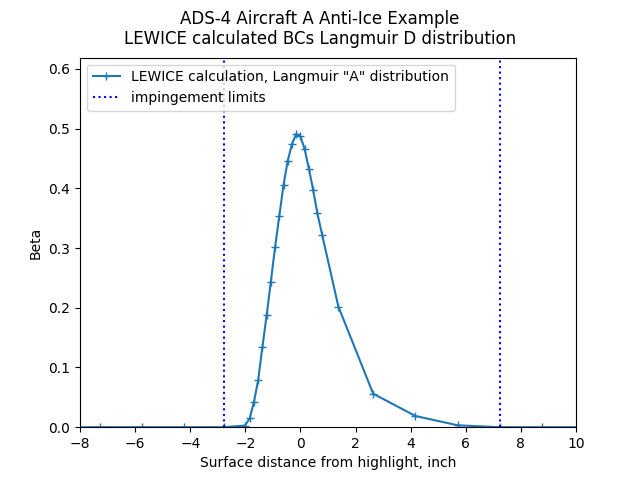
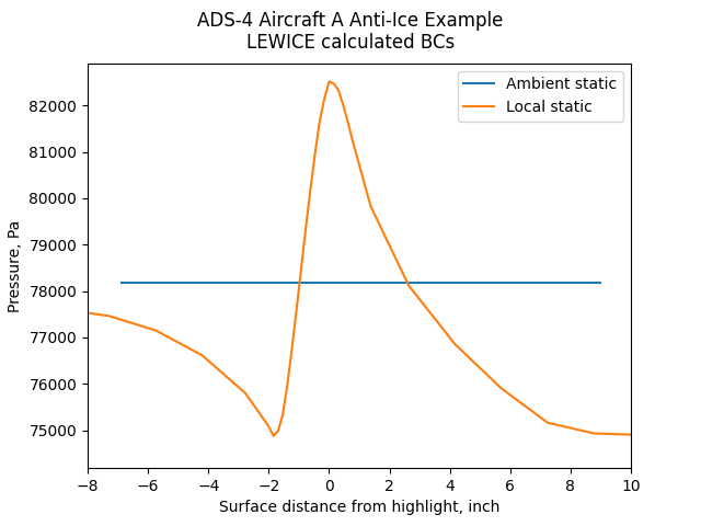
The local pressure, as determined by LEWICE analysis, varies over the heated surface.
The "ambient static" pressure line indicates the surface extent of the heating in the ADS-4 example
(x/c=0.1):
Public domain image by Donald Cook.
The local temperature also varies:
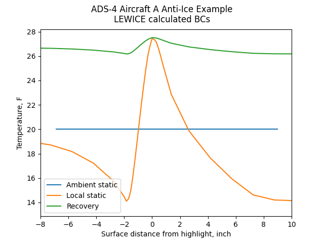
Public domain image by Donald Cook.
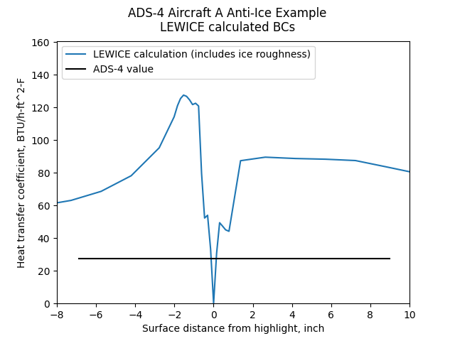
LEWICE also calculates external heat transfer coefficients.
These include the effects of roughness from an initially iced surface
(we will look at the heat transfer coefficients for a non-iced surface in a later section).
Public domain image by Donald Cook.
LEWICE calculates a heat transfer coefficient value of zero at the stagnation point. This is a feature of some integral boundary layer method formulations (the method used in LEWICE).
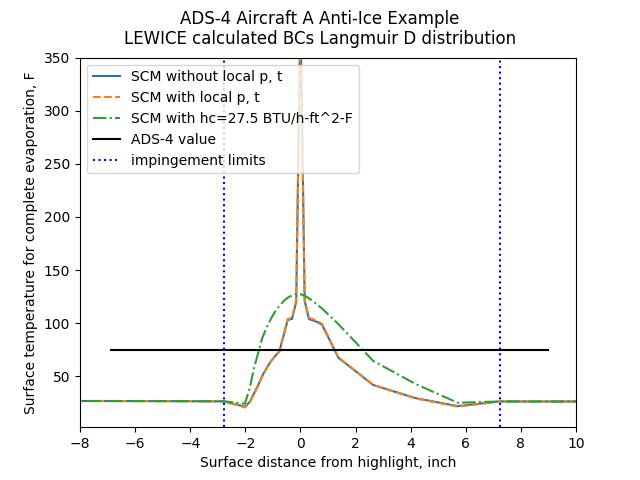
The Standard Computational Model can be used to determine the local heated surface temperature
required to evaporate all impinging water locally.
There is a temperature "spike" at the stagnation line that is caused by
the zero heat transfer coefficient value leading to a non-convergence of the calculation.
Public domain image by Donald Cook.
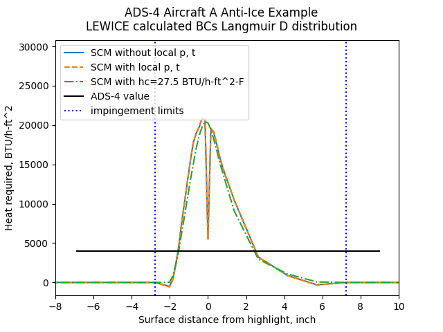
The resulting heat required values:
Public domain image by Donald Cook.
The area under the curve is the total heat required for complete evaporation. This is an ideal, minimal value that assumes that the heat is delivered in the prescribed distribution.
The total heat required values can be compared. The areas under the heating curves are summed up as a function of surface distance.
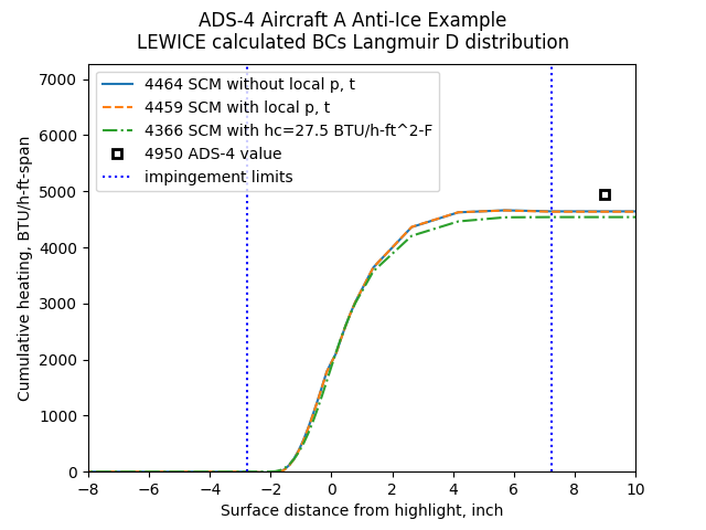
Public domain image by Donald Cook.
The spatially varying boundary conditions had a minor effect on the heat required values for this case. However, at higher Mach values, the variations can be larger.
The ADS-4 value is higher that the other values largely because a wider area of heating was considered (not just within the impingement limits).
Conclusions
With the nominal heat transfer coefficient, the ADS-4 results agree well with those calculated with the Standard Computational Model.
For anti-ice calculations, a 25% change in heat transfer coefficient results in less than a 25% change in heat required.
However, for running wet cases, the result is approximately proportional to the heat transfer coefficient. The average heat transfer coefficient may not well represent the leading edge. The use of the more conservative leading edge cylinder approximation appears to be warranted.
The surface wetness fraction should be included in cases where it is applicable.
Local variations in external pressure and temperature had small effects compared to calculations with constant, averaged values.
Resources
-
"Engineering Summary of Airframe Icing Technical Data", ADS-4 apps.dtic.mil
-
"Ice, Frost, and Rain Protection", AIR1168/4 sae.org
-
"Aircraft Icing Handbook Volume 1", DOT/FAA/CT-88/8-1 apps.dtic.mil
Related
Back to Intermediate Topics